Unit outcomes

By the end of this unit you will be able to:

• Analyse and interpret simple graphs of motion including:
  • displacement–time graphs
  • velocity–time graphs
  • acceleration–time graphs.

What you should know

Before you start this unit, make sure you can:

• Analyse and calculate more problems on motion in one-dimension, using equations of motion:
  • [latex]\scriptsize {{v}_{f}}={{v}_{i}}+a\Delta t[/latex]
  • [latex]\scriptsize s={{v}_{i}}\Delta t+\displaystyle \frac{1}{2}a\Delta {{t}^{2}}[/latex]
  • [latex]\scriptsize v_{f}^{2}=v_{i}^{2}+2as[/latex].

Introduction

In this unit you will learn how to represent horizontal motion graphically, by plotting displacement against time, velocity against time and acceleration against time. Seeing the relationships between quantities graphically will help you to understand the characteristics of different types of motion and how they change over time and help you to put your algebraic calculations into context.

Stationary objects

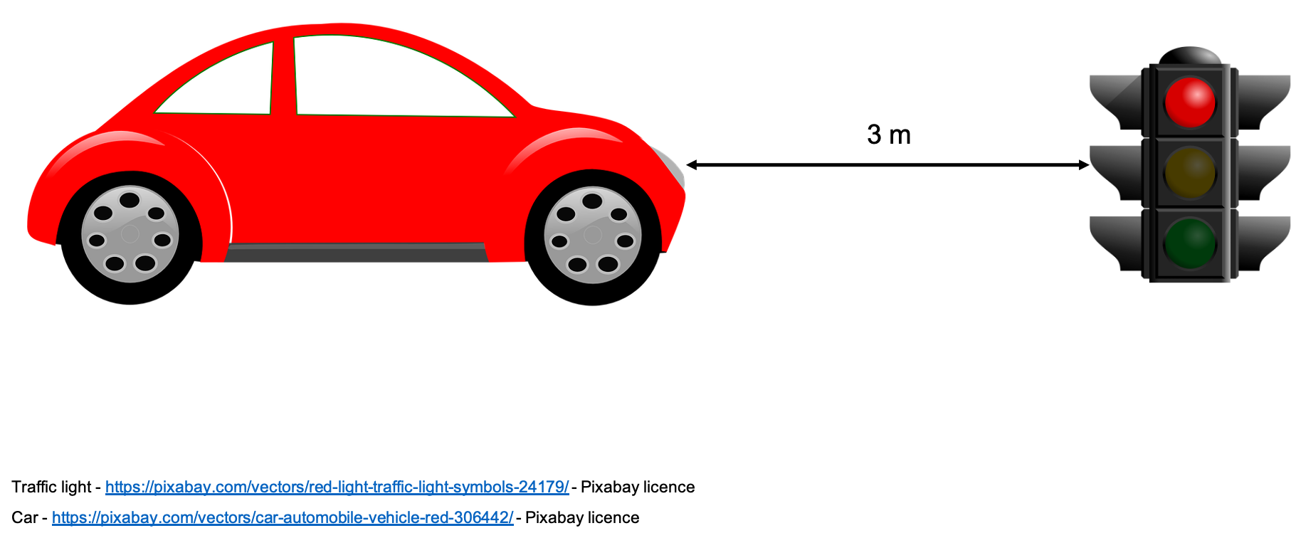
The simplest kind of situation involving motion to investigate is one where there is no motion, where the object in question is stationary. Think about a car waiting at a red traffic light (see figure 1). As time passes, does its position change? If we take the traffic light, which is [latex]\scriptsize 3~\text{m}[/latex] away from the car, as our point of reference, what is the car’s displacement at [latex]\scriptsize t=0\ \text{s}[/latex], [latex]\scriptsize t=10\ \text{s}[/latex], [latex]\scriptsize t=20\ \text{s}[/latex] and [latex]\scriptsize t=30\ \text{s}[/latex]?

We can plot the displacement of the car at each of these times (see figure 2).

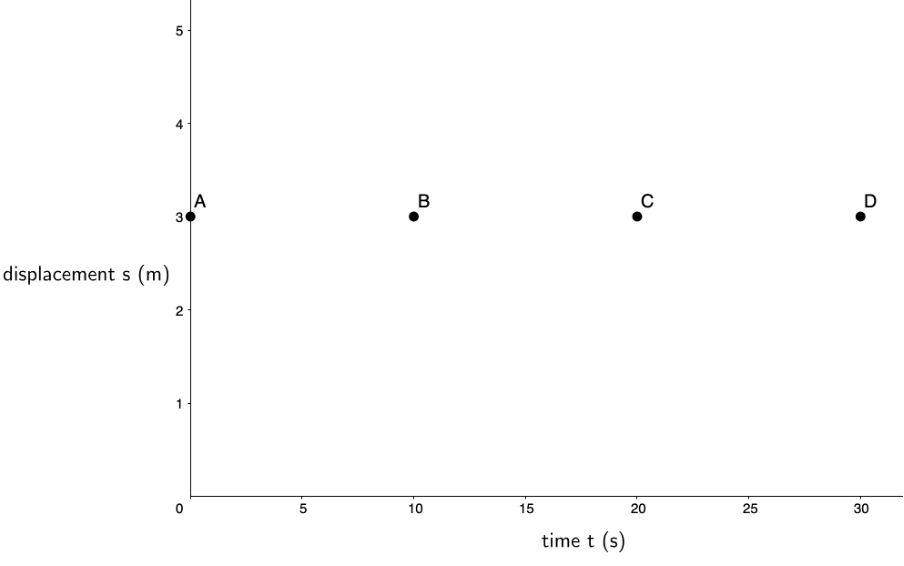
Notice that the independent variable, time, is always on the x-axis while the dependent variable, displacement in this case, is on the y-axis.

Next, we can join these points with a line to indicate that at every time between these points the car’s displacement from the point of reference, the traffic light, is also [latex]\scriptsize 3\ \text{m}[/latex] (see figure 3). When we do this, we produce a displacement–time graph.

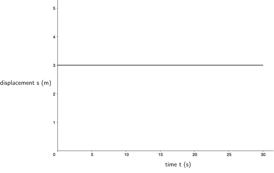
From the graph in figure 3, we can say that the car’s displacement from the point of reference, the traffic light, is [latex]\scriptsize 3\ \text{m}[/latex] and because it remains [latex]\scriptsize 3\ \text{m}[/latex] for the entire period between [latex]\scriptsize t=0\ \text{s}[/latex] and [latex]\scriptsize t=30\ \text{s}[/latex], the car’s velocity during this period is [latex]\scriptsize 0\ \text{m}\text{.}{{\text{s}}^{{-1}}}[/latex]. The car does not move; it is stationary.

What is the gradient of the displacement–time between [latex]\scriptsize t=0\ \text{s}[/latex] and [latex]\scriptsize t=30\ \text{s}[/latex]? Remember that gradient is the change in [latex]\scriptsize y[/latex] divided by the change in [latex]\scriptsize x[/latex].

The change in [latex]\scriptsize y[/latex] is the change in displacement or position, and the change in [latex]\scriptsize x[/latex] is the change in time. Therefore: [latex]\scriptsize \displaystyle m=\displaystyle \frac{{\Delta y}}{{\Delta x}}=\displaystyle \frac{{{{x}_{f}}-{{x}_{i}}}}{{{{t}_{f}}-{{t}_{i}}}}=\displaystyle \frac{{3\ \text{m}-3\ \text{m}}}{{30\ \text{s}-0\ \text{s}}}=\displaystyle \frac{{0\ \text{m}}}{{30\ \text{s}}}=0\ \text{m}\text{.}{{\text{s}}^{{\text{-1}}}}[/latex].

Notice how the gradient of the displacement–time graph is zero, which is the same as the velocity of the car. Also notice how the units for the gradient of a displacement–time graph are [latex]\scriptsize \text{m}\text{.}{{\text{s}}^{{\text{-1}}}}[/latex]. This confirms that the gradient of a displacement time graph tells us what the velocity of the object is.

Take note!

The gradient of a displacement–time graph gives the velocity.

[latex]\scriptsize \displaystyle m=v=\displaystyle \frac{{{{x}_{f}}-{{x}_{i}}}}{{{{t}_{f}}-{{t}_{i}}}}[/latex]

Note: We use [latex]\scriptsize {{x}_{f}}[/latex] and [latex]\scriptsize {{x}_{i}}[/latex] to indicate the final and initial positions

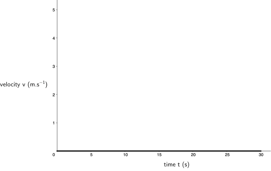
Because the gradient of the displacement–time graph in figure 3 is constant (and zero), we can say that the velocity of the car over this period is also constant (and zero). We can therefore draw a velocity-time graph for the car for the same period (see figure 4). Remember, at each point between [latex]\scriptsize t=0\ \text{s}[/latex] and [latex]\scriptsize t=30\ \text{s}[/latex], the velocity of the car is [latex]\scriptsize 0\ \text{m}\text{.}{{\text{s}}^{{\text{-1}}}}[/latex]. Therefore, the graph is a straight line on the x-axis.

Now, what do you think the gradient of a velocity–time graph tells us about the acceleration of the car? Does the car experience any acceleration during this period?

Let’s work out the gradient of the velocity–time graph in figure 4.

[latex]\scriptsize \displaystyle m=\displaystyle \frac{{\Delta y}}{{\Delta x}}=\displaystyle \frac{{{{v}_{f}}-{{v}_{i}}}}{{{{t}_{f}}-{{t}_{i}}}}=\displaystyle \frac{{0\ \text{m}\text{.}{{\text{s}}^{{-1}}}-0\ \text{m}\text{.}{{\text{s}}^{{-1}}}}}{{30\ \text{s}-0\ \text{s}}}=\displaystyle \frac{{0\ \text{m}\text{.}{{\text{s}}^{{-1}}}}}{{30\ \text{s}}}=0\ \text{m}\text{.}{{\text{s}}^{{\text{-2}}}}[/latex]

Can you see that the gradient of the velocity–time graph gives us the acceleration of the car over the same period? The units of the gradient being [latex]\scriptsize \text{m}\text{.}{{\text{s}}^{{-2}}}[/latex] confirm this.

Take note!

The gradient of a velocity–time graph gives the acceleration.

[latex]\scriptsize \displaystyle m=a=\displaystyle \frac{{{{v}_{f}}-{{v}_{i}}}}{{{{t}_{f}}-{{t}_{i}}}}[/latex]

We know that the car experiences zero acceleration over the entire period. Therefore, we can draw an acceleration–time graph for the car over this period (see figure 5).

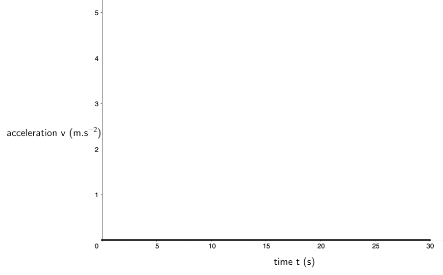
In summary:

• the gradient of a displacement–time graph gives the velocity.
• the gradient of a velocity–time graph gives the acceleration.

Take note!

For a stationary body, there is no change in displacement over time (gradient is constant and zero). Hence the velocity is constant and zero, and the acceleration is constant and zero.

 

Constant velocity

Now let’s consider the slightly more exciting scenario of a car travelling at a constant (non-zero) velocity down the road past a traffic light (our point of reference). Because the car is actually moving, its displacement will be constantly changing. Motion at a constant velocity, or uniform motion, means that the position of the object is changing at a constant rate.

Activity 2.1: Constant velocity

Time required: 15 minutes

What you need:

• a pen or pencil
• a ruler
• a blank piece of paper

What to do:

The displacement from a traffic light of a car at various times is as follows:
[latex]\scriptsize \begin{align*}t&=0\ \text{s}:0\ \text{m}\\t&=5\ \text{s}:10\ \text{m}\\t&=10\ \text{s}:20\ \text{m}\\t&=15\ \text{s}:30\ \text{m}\\t&=20\ \text{s}:40\ \text{m}\end{align*}[/latex]

1. Start by drawing a set of axes on your blank piece of paper. Use about one third of the paper. Label the x-axis as time and the y-axis as displacement. Draw a displacement–time graph using the data above.
2. Determine the gradient of the displacement–time graph. Is the gradient positive, negative or zero? What does this tell you about the velocity of the car over this period?
3. What can you say about the average velocity of the car versus the instantaneous velocity of the car at any point during the period?
4. Use the information in the displacement–time graph and your calculation of its gradient to draw a velocity–time graph for the same time period. Use about one third of your paper for this graph.
5. Determine the gradient of the velocity–time graph. What does this tell you about the acceleration of the car over this period?
6. Use the information in the velocity–time graph and your calculation of its gradient to draw an acceleration–time graph for the same time period. Use about one third of your paper for this graph.
7. Go back your velocity–time graph. Determine the area under the graph between [latex]\scriptsize t=0\ \text{s}[/latex] and [latex]\scriptsize t=20\ \text{s}[/latex]. What do you think this area tells you?

What did you find?

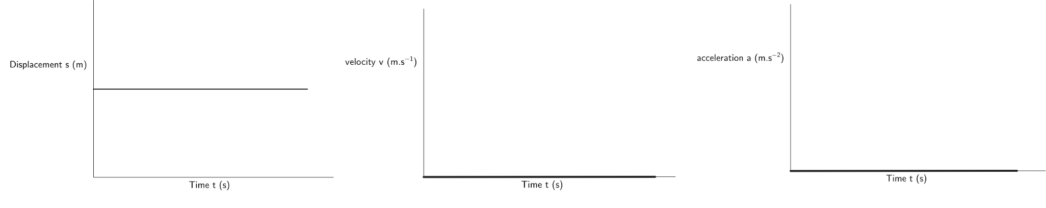
1. Here is the displacement–time graph of the given data. The individual data points have been joined to form a straight line.
   
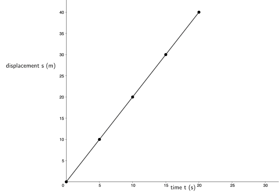
2. Because the displacement–time graph is a straight line, we know that its gradient is the same at any point on the line. Therefore, we can measure the change in [latex]\scriptsize y[/latex] and the corresponding change in [latex]\scriptsize x[/latex] between any two points on the line. In the calculation which follows, we have chosen to measure the gradient between the first point and the last point.
   .
   [latex]\scriptsize \displaystyle m=\displaystyle \frac{{\Delta y}}{{\Delta x}}=\displaystyle \frac{{{{x}_{f}}-{{x}_{i}}}}{{{{t}_{f}}-{{t}_{i}}}}=\displaystyle \frac{{40\ \text{m}-0\ \text{m}}}{{20\ \text{s}-0\ \text{s}}}=\displaystyle \frac{{40\ \text{m}\text{.}{{\text{s}}^{{-1}}}}}{{20\ \text{s}}}=2\ \text{m}\text{.}{{\text{s}}^{{\text{-1}}}}[/latex]
   .
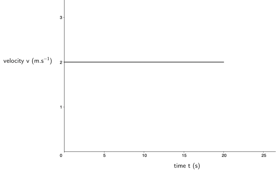
   This means that the velocity of the car over the time period is [latex]\scriptsize \displaystyle 2\ \text{m}\text{.}{{\text{s}}^{{\text{-1}}}}[/latex]. The gradient of the line is therefore not zero but a positive value. Positive gradients slope up from left to right. A positive gradient indicates a positive velocity. Therefore, a negative displacement–time graph gradient (sloping down from left to right) would indicate a negative velocity.
3. Because the gradient of the displacement–time graph is constant, it means that the velocity of the car is also constant over the period. Therefore, the average velocity of the car ([latex]\scriptsize \displaystyle 2\ \text{m}\text{.}{{\text{s}}^{{\text{-1}}}}[/latex]) is the same as the instantaneous velocity of the car at any point over the period (also [latex]\scriptsize \displaystyle 2\ \text{m}\text{.}{{\text{s}}^{{\text{-1}}}}[/latex]).
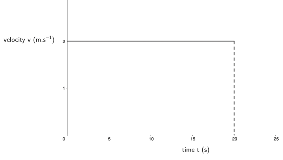
4. Here is the velocity–time graph for the same period. The velocity of the car is a constant [latex]\scriptsize \displaystyle 2\ \text{m}\text{.}{{\text{s}}^{{\text{-1}}}}[/latex].
   
5. [latex]\scriptsize \displaystyle m=\displaystyle \frac{{\Delta y}}{{\Delta x}}=\displaystyle \frac{{{{v}_{f}}-{{v}_{i}}}}{{{{t}_{f}}-{{t}_{i}}}}=\displaystyle \frac{{2\ \text{m}\text{.}{{\text{s}}^{{-1}}}-2\ \text{m}\text{.}{{\text{s}}^{{-1}}}}}{{20\ \text{s}-0\ \text{s}}}=\displaystyle \frac{{0\ \text{m}\text{.}{{\text{s}}^{{-1}}}}}{{20\ \text{s}}}=0\ \text{m}\text{.}{{\text{s}}^{{\text{-2}}}}[/latex]
   The gradient of the velocity–time graph is [latex]\scriptsize \displaystyle 0\ \text{m}\text{.}{{\text{s}}^{{\text{-2}}}}[/latex]. Therefore, the acceleration is a constant [latex]\scriptsize \displaystyle 0\ \text{m}\text{.}{{\text{s}}^{{\text{-2}}}}[/latex] over the period.
6. The acceleration over the period is constant and zero. Therefore, this is the acceleration–time graph:
   
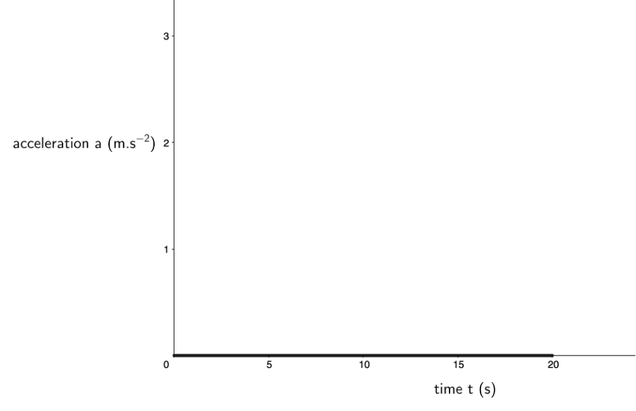
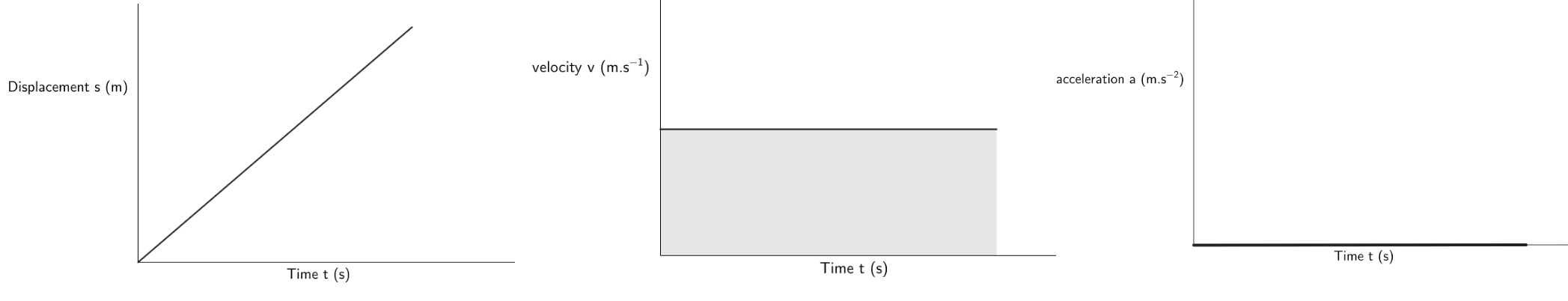
7. The area under the velocity–time graph between [latex]\scriptsize t=0\ \text{s}[/latex] and [latex]\scriptsize t=20\ \text{s}[/latex] forms a rectangle with a length of [latex]\scriptsize \displaystyle 20\ \text{s}[/latex] and a height of [latex]\scriptsize \displaystyle 2\ \text{m}\text{.}{{\text{s}}^{{\text{-1}}}}[/latex]. Therefore, the area is [latex]\scriptsize \displaystyle 20\ \text{s}\times 2\ \text{m}\text{.}{{\text{s}}^{{\text{-1}}}}=40\ \text{m}[/latex]. The area under the velocity–time graph is the same as the total displacement of the car over the period ([latex]\scriptsize \displaystyle 40\ \text{m}[/latex]). The units of this calculation also support the conclusion that the area under a velocity–time graph gives us the displacement.
   

In activity 2.1 we confirmed the fact that:

• the gradient of a displacement–time graph gives the velocity
• the gradient of a velocity–time graph gives the acceleration.

We have also discovered the following:

• a positive gradient (sloping up from left to right) indicates a positive velocity or acceleration
• the area under a velocity–time graph gives the displacement.

Take note!

For a body with constant velocity (zero acceleration), there is a constant change in displacement over time (gradient is constant but non-zero). Therefore, velocity is constant and non-zero, and acceleration is constant and zero.

The area under the velocity–time graph gives the displacement.

 

What do you think the area under an acceleration–time graph gives us?

Constant acceleration

In the previous section we dealt with uniform motion, where an object moves at a uniform or constant velocity. Because the velocity is constant, the acceleration is zero. But what happens when the acceleration is constant but not zero. In other words, what do the three graphs look like for an object that is experiencing a constant non-zero acceleration?

Let’s consider a car pulling away from a traffic light under constant acceleration.

Activity 2.2: Constant acceleration

Time required: 15 minutes

What you need:

• a pen or pencil
• a ruler
• a blank piece of paper

What to do:

The velocity of a car at various times is as follows:

[latex]\scriptsize \begin{align*}t&=0\ \text{s}:0\ \text{m}\text{.}{{\text{s}}^{{-1}}}\\t&=1\ \text{s}:5\ \text{m}\text{.}{{\text{s}}^{{-1}}}\\t&=2\ \text{s}:10\ \text{m}\text{.}{{\text{s}}^{{-1}}}\\t&=3\ \text{s}:15\ \text{m}\text{.}{{\text{s}}^{{-1}}}\\t&=4\ \text{s}:20\ \text{m}\text{.}{{\text{s}}^{{-1}}}\end{align*}[/latex]

1. Start by drawing a set of axes on your blank piece of paper. Use about one third of the paper. Label the x-axis as time and the y-axis as velocity. Draw a velocity–time graph using the data above.
2. Is the graph a straight line? Is the gradient constant? Is it positive or negative? What does this tell you about the acceleration? Determine the acceleration of the car from your velocity–time graph.
3. What can you say about the average acceleration of the car versus the instantaneous acceleration of the car at any point during the period?
4. Use the information in the velocity–time graph and your calculation of its gradient to draw an acceleration–time graph for the same time period. Use about one third of your paper for this graph.
5. Determine the area under the acceleration–time graph between [latex]\scriptsize t=0\ \text{s}[/latex] and [latex]\scriptsize t=4\ \text{s}[/latex]. How does this relate to the velocity of the car?
6. Use the area under the velocity–time graph over each second of the whole period to draw a displacement–time graph for the whole time period. Use about one third of your paper for this graph.
7. Is the displacement–time graph a straight line? Is its gradient constant? What does this tell you about the velocity of the car?

What did you find?

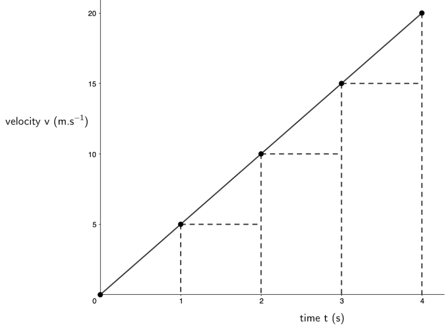
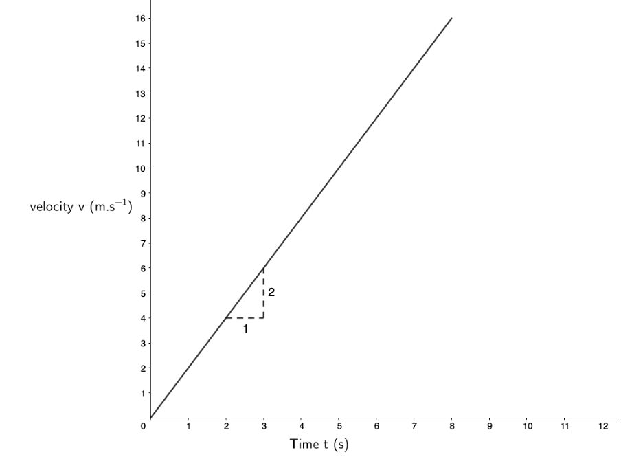
1. Here is the velocity–time graph of the given data:
   
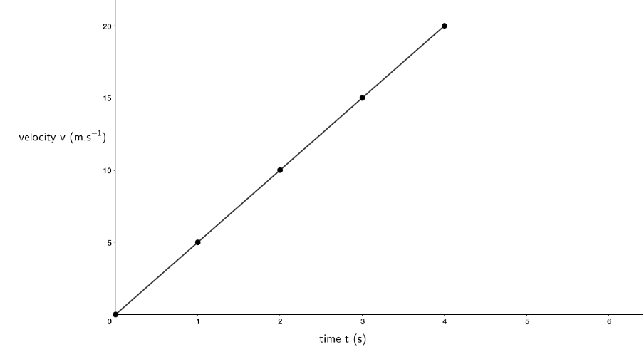
2. The graph is a straight line. It has a constant positive gradient. Therefore, the acceleration of the car is constant and positive. [latex]\scriptsize \displaystyle m=a=\displaystyle \frac{{{{v}_{f}}-{{v}_{i}}}}{{{{t}_{f}}-{{t}_{i}}}}=\displaystyle \frac{{5\ \text{m}\text{.}{{\text{s}}^{{-1}}}-0\ \text{m}\text{.}{{\text{s}}^{{-1}}}}}{{1\ \text{s}-0\ \text{s}}}=\displaystyle \frac{{5\ \text{m}\text{.}{{\text{s}}^{{-1}}}}}{{1\ \text{s}}}=5\ \text{m}\text{.}{{\text{s}}^{{\text{-2}}}}[/latex]
3. Because the gradient of the velocity–time graph is the same in all places, the average acceleration of the car is equal to the instantaneous acceleration of the car at any point over the period.
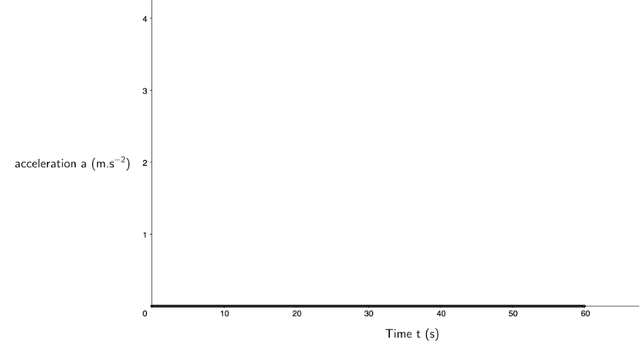
4. The acceleration of the car over the period is a constant [latex]\scriptsize 5\ \text{m}\text{.}{{\text{s}}^{{\text{-1}}}}[/latex]. Therefore, the acceleration–time graph is as follows:
   
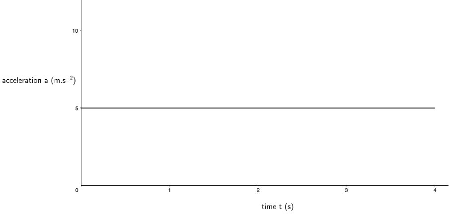
5. The area under the acceleration–time graph between [latex]\scriptsize t=0\ \text{s}[/latex] and [latex]\scriptsize t=4\ \text{s}[/latex] is a rectangle with a length of [latex]\scriptsize 4\ \text{s}[/latex] and a height of [latex]\scriptsize 5\ \text{m}\text{.}{{\text{s}}^{{-2}}}[/latex]. The area of this rectangle is [latex]\scriptsize \displaystyle 4\ \text{s}\times 5\ \text{m}\text{.}{{\text{s}}^{{-2}}}=20\ \text{m}\text{.}{{\text{s}}^{{-1}}}[/latex]. This is the same as the final velocity of the car at the end of the period.
6. We first need to determine the area under the velocity–time graph for each [latex]\scriptsize 1\ \text{s}[/latex] slice of time. Each slice can be divided into a right-angled triangle and a rectangle.
   .
   
   .
   The areas for each slice are as follows:[latex]\scriptsize \begin{align*}t&=0\ \text{s to }t=1\ \text{s}:\displaystyle \frac{1}{2}\times 1\ \text{s}\times 5\ \text{m}\text{.}{{\text{s}}^{{\text{-1}}}}=2.5\ \text{m}\\t&=1\ \text{s to }t=2\ \text{s}:\displaystyle \frac{1}{2}\times 1\ \text{s}\times 5\ \text{m}\text{.}{{\text{s}}^{{\text{-1}}}}+1\ \text{s}\times 5\ \text{m}\text{.}{{\text{s}}^{{\text{-1}}}}=7.5\ \text{m}\\t&=2\ \text{s to }t=3\ \text{s}:\displaystyle \frac{1}{2}\times 1\ \text{s}\times 5\ \text{m}\text{.}{{\text{s}}^{{\text{-1}}}}+1\ \text{s}\times 10\ \text{m}\text{.}{{\text{s}}^{{\text{-1}}}}=12.5\ \text{m}\\t&=3\ \text{s to }t=4\ \text{s}:\displaystyle \frac{1}{2}\times 1\ \text{s}\times 5\ \text{m}\text{.}{{\text{s}}^{{\text{-1}}}}+1\ \text{s}\times 15\ \text{m}\text{.}{{\text{s}}^{{\text{-1}}}}=17.5\ \text{m}\end{align*}[/latex]
   .
   After the first second, the total displacement is [latex]\scriptsize 2.5\ \text{m}[/latex].
   After the second second, the total displacement is [latex]\scriptsize 2.5\ \text{m}+7.5\ \text{m}=10\ \text{m}[/latex].
   After the third second, the total displacement is [latex]\scriptsize 2.5\ \text{m}+7.5\ \text{m}+12.5\ \text{m}=22.5\ \text{m}[/latex].
   After the fourth second, the total displacement is [latex]\scriptsize 2.5\ \text{m}+7.5\ \text{m}+12.5\ \text{m}+17.5\ \text{m}=40\ \text{m}[/latex].
   .
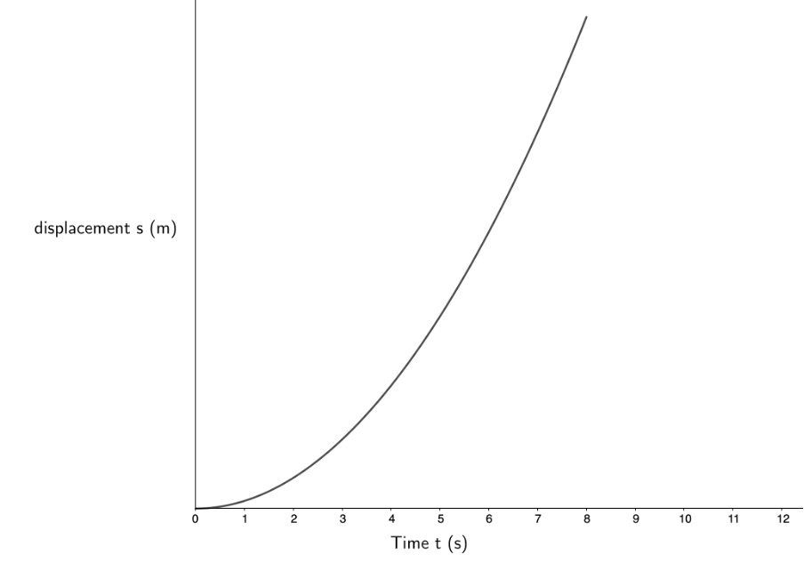
   We can now draw the displacement–time graph:
   
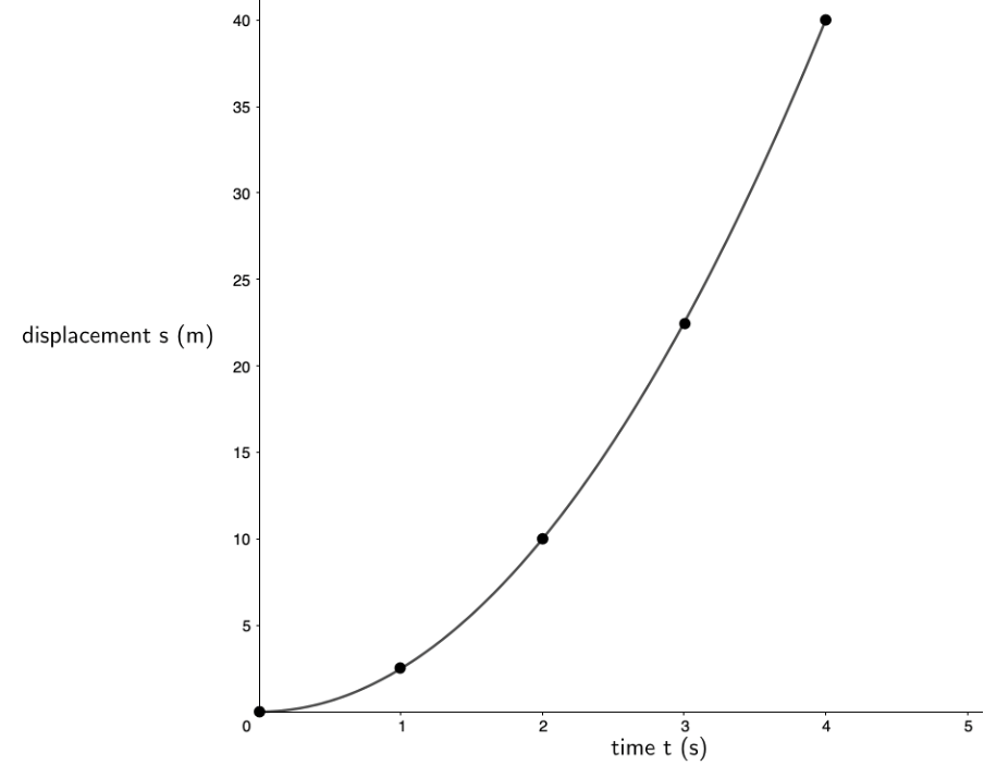
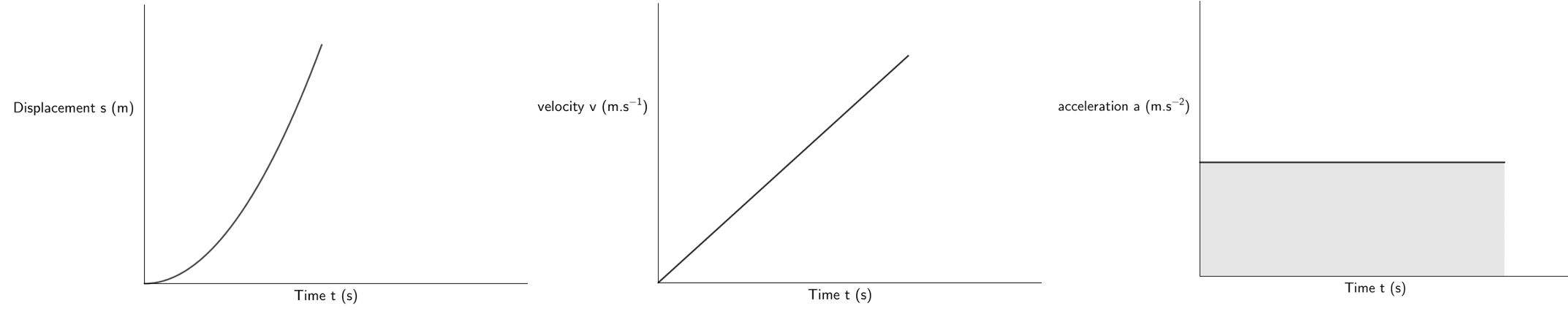
7. The displacement–time graph is not a straight line. Its gradient is, therefore, not constant. Its gradient gets steeper and steeper as time goes on. If the gradient of a displacement–time graph gives us velocity, then this means that the velocity increases as time goes on which is exactly what is happening. Remember the car is accelerating which means that the velocity is constantly increasing.

Once again, we have seen how the gradient of a displacement–time graph gives the velocity and the gradient of a velocity–time graph gives the acceleration. If a displacement–time graph is a straight line, the gradient is constant meaning that the velocity is constant. If a velocity–time graph is a straight line, the gradient is constant, meaning that the acceleration is constant.

If a displacement–time graph is not a straight line, the gradient is not constant, and the velocity is changing (the body is accelerating).

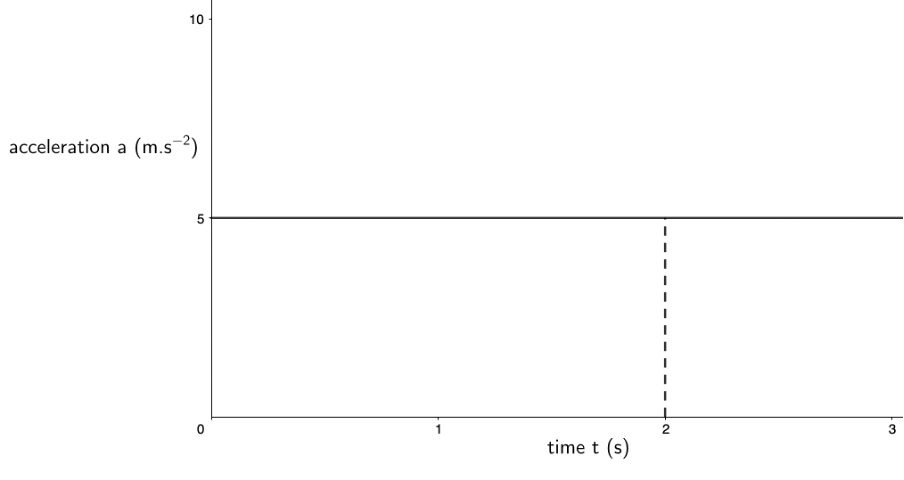
Just as we used a velocity–time graph to find displacement, we can use an acceleration–time graph to find the velocity of an object at a given moment in time. We simply calculate the area under the acceleration–time graph, at a given time. In figure 8, which shows an object at a constant positive acceleration, the increase in velocity of the object after two seconds corresponds to the area of the rectangle under the graph between [latex]\scriptsize t=0\ \text{s}[/latex] and [latex]\scriptsize t=2\ \text{s}[/latex].

Take note!

For a body with constant non-zero acceleration, there is a constant change in velocity over time (the gradient is constant but non-zero). Therefore, acceleration is constant and non-zero. Displacement changes over time but at a non-constant rate (the graph is not a straight line and does not have a constant gradient).

The area under the acceleration–time graph gives the velocity.

 

Interpreting graphs of motion

There are two types of questions that you will need to be able to answer. The first requires you to read and interpret given graphs of motion. The second requires you to draw your own graphs of motion based on information given, either in words or in the form of a graph of motion.

Example 2.1

A radio-controlled car drives along a straight track. The following displacement–time graph was produced:

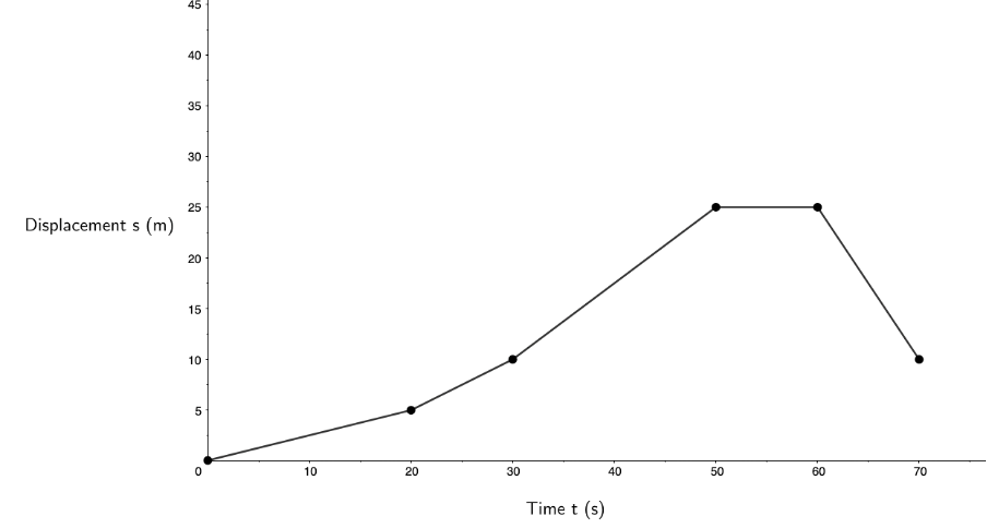
1. Calculate the velocity of the car between [latex]\scriptsize 30\ \text{s}[/latex] and [latex]\scriptsize 50\ \text{s}[/latex].
2. Calculate the velocity of the car between [latex]\scriptsize 0\ \text{s}[/latex] and [latex]\scriptsize 20\ \text{s}[/latex].
3. During which period was the car driving the fastest? Explain.
4. During which period was the car stationary? Explain.
5. Did the car ever reverse? If so, when? Explain.

Solutions

1. The velocity of the car between [latex]\scriptsize 30\ \text{s}[/latex] and [latex]\scriptsize 50\ \text{s}[/latex] is the gradient of the line between [latex]\scriptsize t=30\ \text{s}[/latex] and [latex]\scriptsize t=50\ \text{s}[/latex].
   .
   [latex]\scriptsize \displaystyle m=v=\displaystyle \frac{{{{x}_{f}}-{{x}_{i}}}}{{{{t}_{f}}-{{t}_{i}}}}=\displaystyle \frac{{25\ \text{m}-10\ \text{m}}}{{50\ \text{s}-30\ \text{s}}}=\displaystyle \frac{{15\ \text{m}}}{{20\ \text{s}}}=0.75\ \text{m}\text{.}{{\text{s}}^{{\text{-1}}}}[/latex]
   .
   The velocity of the car between [latex]\scriptsize 30\ \text{s}[/latex] and [latex]\scriptsize 50\ \text{s}[/latex] is [latex]\scriptsize 0.75\ \text{m}\text{.}{{\text{s}}^{{-1}}}[/latex].
2. The velocity of the car between [latex]\scriptsize 0\ \text{s}[/latex] and [latex]\scriptsize 20\ \text{s}[/latex] is the gradient of the line between [latex]\scriptsize t=0\ \text{s}[/latex] and [latex]\scriptsize t=20\ \text{s}[/latex].
   .
   [latex]\scriptsize \displaystyle m=v=\displaystyle \frac{{{{x}_{f}}-{{x}_{i}}}}{{{{t}_{f}}-{{t}_{i}}}}=\displaystyle \frac{{5\ \text{m}-0\ \text{m}}}{{20\ \text{s}-0\ \text{s}}}=\displaystyle \frac{{5\ \text{m}}}{{20\ \text{s}}}=0.25\ \text{m}\text{.}{{\text{s}}^{{\text{-1}}}}[/latex]
   .
   The velocity of the car between [latex]\scriptsize 0\ \text{s}[/latex] and [latex]\scriptsize 20\ \text{s}[/latex] is [latex]\scriptsize 0.25\ \text{m}\text{.}{{\text{s}}^{{-1}}}[/latex].
3. The period between [latex]\scriptsize 30\ \text{s}[/latex] and [latex]\scriptsize 50\ \text{s}[/latex] has the steepest gradient. Therefore, this is when the car was driving the fastest.
4. The period between [latex]\scriptsize 50\ \text{s}[/latex] and [latex]\scriptsize 60\ \text{s}[/latex] has a gradient of zero indicating zero velocity. This is when the car was stationary.
5. Between [latex]\scriptsize 60\ \text{s}[/latex] and [latex]\scriptsize 70\ \text{s}[/latex], we see that the displacement of the car decreased (the car got closer to where it had started). We can also see that during this period, the gradient of the graph is negative which indicates a negative velocity. Both of these facts indicate that in this period the car reversed. It decreased its displacement by travelling backwards. A negative velocity also indicates that the velocity (and hence motion) of the car was in the opposite direction to before, i.e. reversing.

Example 2.2

The following velocity–time graph shows the motion of a drone taking off from the ground at [latex]\scriptsize t=0\ \text{s}[/latex] and flying vertically up. Take upwards to be the positive direction.

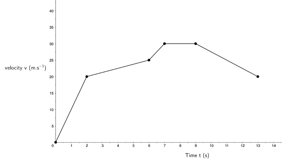
1. Describe the motion of the drone between [latex]\scriptsize t=0\ \text{s}[/latex] and [latex]\scriptsize t=2\ \text{s}[/latex].
2. What is the acceleration of the drone between [latex]\scriptsize 2\ \text{s}[/latex] and [latex]\scriptsize 6\ \text{s}[/latex]?
3. When was the drone’s acceleration zero?
4. Did the drone ever decelerate? If so, when?
5. Describe the motion of the drone between [latex]\scriptsize 6\ \text{s}[/latex] and [latex]\scriptsize 13\ \text{s}[/latex].
6. What was the drone’s maximum velocity?
7. Did the drone ever fly downwards?
8. How high off the ground is the drone after the first [latex]\scriptsize 6\ \text{s}[/latex]?
9. Draw an acceleration–time graph for the period [latex]\scriptsize 0\ \text{s}[/latex] and [latex]\scriptsize 13\ \text{s}[/latex].

Solutions

1. As the velocity during this period was positive, this means that the drone took off and flew vertically up with a constant acceleration equal to the gradient of the graph between [latex]\scriptsize t=0\ \text{s}[/latex] and [latex]\scriptsize t=2\ \text{s}[/latex].
2. [latex]\scriptsize \displaystyle m=a=\displaystyle \frac{{{{v}_{f}}-{{v}_{i}}}}{{{{t}_{f}}-{{t}_{i}}}}=\displaystyle \frac{{25\ \text{m}\text{.}{{\text{s}}^{{-1}}}-20\ \text{m}\text{.}{{\text{s}}^{{-1}}}}}{{6\ \text{s}-2\ \text{s}}}=\displaystyle \frac{{5\ \text{m}\text{.}{{\text{s}}^{{-1}}}}}{{4\ \text{s}}}=1.25\ \text{m}\text{.}{{\text{s}}^{{\text{-2}}}}[/latex]
3. The change in velocity of the drone was zero between [latex]\scriptsize 7\ \text{s}[/latex] and [latex]\scriptsize 9\ \text{s}[/latex] (the gradient of the line is zero). Therefore, its acceleration during this period was zero.
4. Between [latex]\scriptsize 9\ \text{s}[/latex] and [latex]\scriptsize 13\ \text{s}[/latex], the gradient of the velocity–time graph was negative (its change in velocity was negative). Therefore, during this period the drone decelerated.
5. Between [latex]\scriptsize 6\ \text{s}[/latex] and [latex]\scriptsize 7\ \text{s}[/latex] the drone accelerated from [latex]\scriptsize 25\ \text{m}\text{.}{{\text{s}}^{{\text{-1}}}}[/latex] to [latex]\scriptsize 30\ \text{m}\text{.}{{\text{s}}^{{\text{-1}}}}[/latex]. Then it travelled at a constant velocity of [latex]\scriptsize 30\ \text{m}\text{.}{{\text{s}}^{{\text{-1}}}}[/latex] between [latex]\scriptsize 7\ \text{s}[/latex] and [latex]\scriptsize 9\ \text{s}[/latex]. Then it decelerated from [latex]\scriptsize 30\ \text{m}\text{.}{{\text{s}}^{{\text{-1}}}}[/latex] to [latex]\scriptsize 20\ \text{m}\text{.}{{\text{s}}^{{\text{-1}}}}[/latex] between [latex]\scriptsize 9\ \text{s}[/latex] and [latex]\scriptsize 13\ \text{s}[/latex].
6. The greatest velocity shown on the graph is [latex]\scriptsize 30\ \text{m}\text{.}{{\text{s}}^{{\text{-1}}}}[/latex]. This is the drone’s maximum velocity.
7. At no point does the graph represent a negative velocity. Therefore, at no time did the drone fly downwards.
8. The drone’s displacement after [latex]\scriptsize 6\ \text{s}[/latex] is equal to the area under the velocity–time graph between [latex]\scriptsize t=0\ \text{s}[/latex] and [latex]\scriptsize t=6\ \text{s}[/latex].
   This area can be divided up as follows:
   
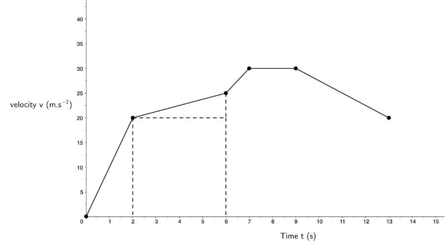
   This area is calculated as follows:
   [latex]\scriptsize \left( {\displaystyle \frac{1}{2}\times 2\ \text{s}\times 20\ \text{m}\text{.}{{\text{s}}^{{\text{-1}}}}} \right)+\left( {4\ \text{s}\times 20\ \text{m}\text{.}{{\text{s}}^{{\text{-1}}}}} \right)+\left( {\displaystyle \frac{1}{2}\times 4\ \text{s}\times 5\ \text{m}\text{.}{{\text{s}}^{{\text{-1}}}}} \right)=110\ \text{m}[/latex]
   The drone will be [latex]\scriptsize 110\ \text{m}[/latex]off the ground after the first [latex]\scriptsize 6\ \text{s}[/latex].
9. To draw the corresponding acceleration–time graph, we need to calculate the gradient of each part of the velocity–time graph. These gradients are as follows:
   [latex]\scriptsize \displaystyle \begin{align*}t&=0\ \text{s to }t=2\ \text{s}:10\ \text{m}\text{.}{{\text{s}}^{{\text{-2}}}}\\t&=2\ \text{s to }t=6\ \text{s}:1.25\ \text{m}\text{.}{{\text{s}}^{{\text{-2}}}}\\t&=6\ \text{s to }t=7\ \text{s}:5\ \text{m}\text{.}{{\text{s}}^{{\text{-2}}}}\\t&=7\ \text{s to }t=9\ \text{s}:0\ \text{m}\text{.}{{\text{s}}^{{\text{-2}}}}\\t&=9\ \text{s to }t=13\ \text{s}:m=\displaystyle \frac{{{{v}_{f}}-{{v}_{i}}}}{{{{t}_{f}}-{{t}_{i}}}}=\displaystyle \frac{{20\ \text{m}\text{.}{{\text{s}}^{{-1}}}-30\ \text{m}\text{.}{{\text{s}}^{{-1}}}}}{{13\ \text{s}-9\ \text{s}}}=\displaystyle \frac{{10\ \text{m}\text{.}{{\text{s}}^{{-1}}}}}{{4\ \text{s}}}-2.5\ \text{m}\text{.}{{\text{s}}^{{\text{-2}}}}\end{align*}[/latex]
   .
   Note: The final gradient is negative indicating deceleration.
   .
   In all cases, the gradients are constant over the periods, indicating constant accelerations (i.e. flat acceleration–time graphs). Notice how we need to extend the y-axis to accommodate the period of negative acceleration (deceleration).
   .
   

Exercise 2.1

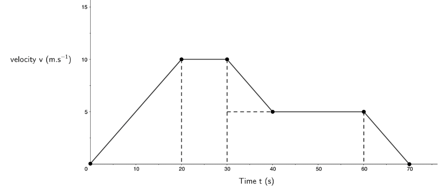
1. The velocity–time graph of a cyclist is shown below:
   
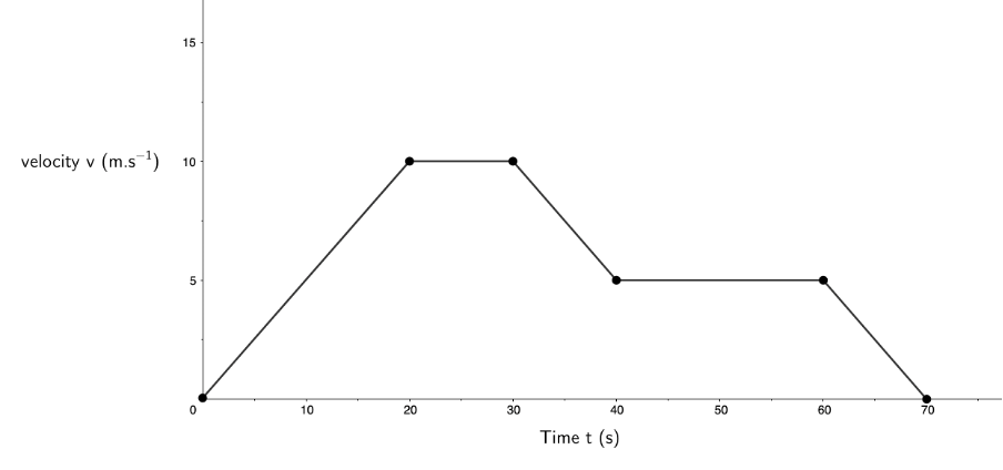
   1. What is the cyclist’s acceleration for the first [latex]\scriptsize 20\ \text{s}[/latex]?
   2. During which period(s) is the cyclist not accelerating?
   3. Calculate the total displacement of the cyclist after [latex]\scriptsize 60\ \text{s}[/latex].
   4. What is the cyclist’s average velocity over the first [latex]\scriptsize 60\ \text{s}[/latex]?
   5. Describe the cyclist’s motion at [latex]\scriptsize t=70\ \text{s}[/latex].
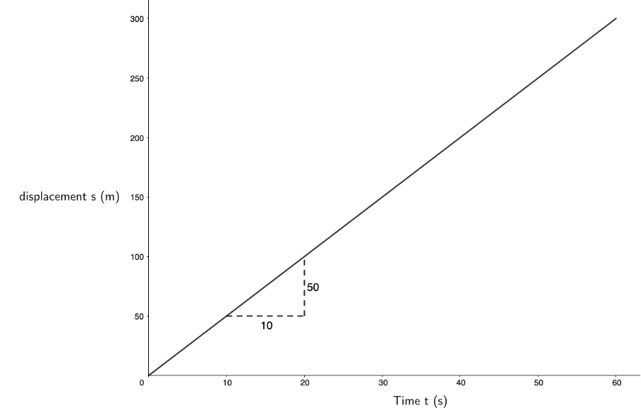
2. The following displacement–time graph describes the motion of an athlete:
   
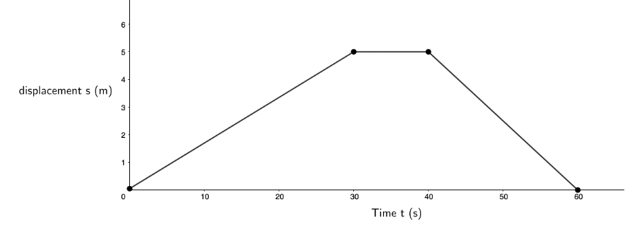
   1. What is the athlete’s velocity during the first [latex]\scriptsize 15\ \text{s}[/latex]?
   2. What is the velocity of the athlete from [latex]\scriptsize t=30\ \text{s}[/latex] to [latex]\scriptsize t=40\ \text{s}[/latex]?
   3. What is the velocity of the athlete for the last [latex]\scriptsize 20\ \text{s}[/latex]?
   4. What is the athlete’s total displacement? Provide a description of the possible motion of this athlete in the real world.

The full solutions can be found at the end of the unit.

Summary

In this unit you have learnt the following:

• The gradient of a displacement–time graph gives velocity.
• The gradient of a velocity–time graph gives acceleration.
• The area under an acceleration–time graph gives velocity.
• The area under a velocity–time graph gives displacement.

Unit 2: Assessment

Suggested time to complete: 30 minutes

1. A cyclist cycles with a constant acceleration of [latex]\scriptsize 2\ \text{m}\text{.}{{\text{s}}^{{-2}}}[/latex] for [latex]\scriptsize 8\ \text{s}[/latex]. Draw the acceleration–time, velocity–time and displacement–time graphs for the motion. Accurate values are only needed for the acceleration–time and velocity–time graphs.
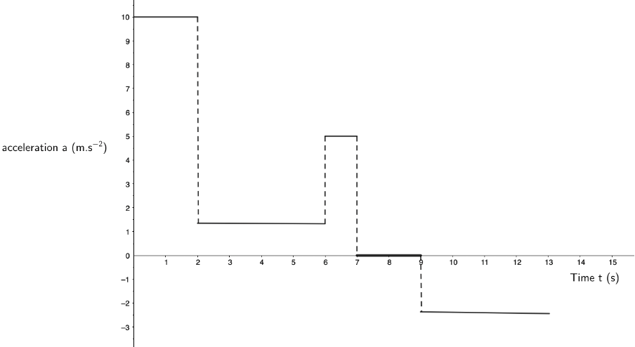
2. The following velocity–time graph describes the motion of a car:
   
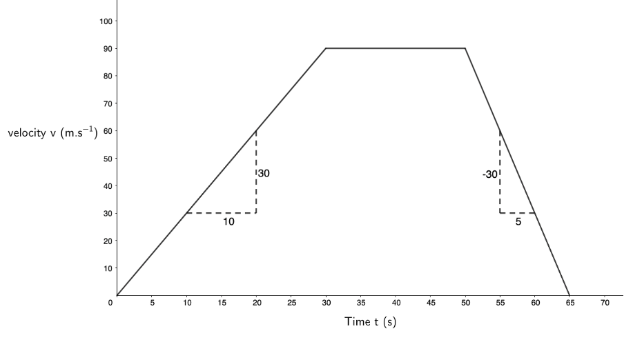
   Draw the corresponding displacement–time and acceleration–time graphs and explain the motion of the car according to the three graphs.
3. A racing car starts from rest at a pit stop and accelerates at a rate of [latex]\scriptsize 3\ \text{m}\text{.}{{\text{s}}^{{-2}}}[/latex] for [latex]\scriptsize 30\ \text{s}[/latex]. It then travels at a constant speed for [latex]\scriptsize 20\ \text{s}[/latex] and slows down at a rate of [latex]\scriptsize 6\ \text{m}\text{.}{{\text{s}}^{{-2}}}[/latex] until it comes to a stop.
   1. Draw a velocity–time graph for the motion of the racing car. Indicate ALL details on the graph.
   2. From the graph, what is the velocity of the racing car after [latex]\scriptsize 30\ \text{s}[/latex]?
   3. From the graph, determine the total distance covered by the racing car.

The full solutions can be found at the end of the unit.

Unit 2: Solutions

Exercise 2.1

1. .
   1. [latex]\scriptsize \displaystyle m=a=\displaystyle \frac{{{{v}_{f}}-{{v}_{i}}}}{{{{t}_{f}}-{{t}_{i}}}}=\displaystyle \frac{{10\ \text{m}\text{.}{{\text{s}}^{{-1}}}-0\ \text{m}\text{.}{{\text{s}}^{{-1}}}}}{{20\ \text{s}-0\ \text{s}}}=\displaystyle \frac{{10\ \text{m}\text{.}{{\text{s}}^{{-1}}}}}{{20\ \text{s}}}=0.5\ \text{m}\text{.}{{\text{s}}^{{\text{-2}}}}[/latex]
   2. Between [latex]\scriptsize t=20\ \text{s}[/latex] and [latex]\scriptsize t=30\ \text{s}[/latex] and between [latex]\scriptsize t=40\ \text{s}[/latex] and [latex]\scriptsize t=60\ \text{s}[/latex] the gradient of the graph is zero indicating no change in velocity and, hence, no acceleration.
   3. We can divide the area under the graph between [latex]\scriptsize t=0\ \text{s}[/latex] and [latex]\scriptsize t=60\ \text{s}[/latex] up as follows.
      
      The total area is:
      [latex]\scriptsize \left( {\displaystyle \frac{1}{2}\times 20\ \text{s}\times 10\ \text{m}\text{.}{{\text{s}}^{{\text{-1}}}}} \right)+\left( {10\ \text{s}\times 10\ \text{m}\text{.}{{\text{s}}^{{\text{-1}}}}} \right)+\left( {\displaystyle \frac{1}{2}\times 10\ \text{s}\times 5\ \text{m}\text{.}{{\text{s}}^{{\text{-1}}}}} \right)+\left( {30\ \text{s}\times 5\ \text{m}\text{.}{{\text{s}}^{{\text{-1}}}}} \right)=375\ \text{m}[/latex]
      Therefore, the cyclist’s total displacement after the first [latex]\scriptsize 60\ \text{s}[/latex] is [latex]\scriptsize 375\ \text{m}[/latex].
   4. [latex]\scriptsize {{v}_{{avg}}}=\displaystyle \frac{{\Delta s}}{{\Delta t}}=\displaystyle \frac{{375\ \text{m}}}{{60\ \text{s}}}=6.25\ \text{m}\text{.}{{\text{s}}^{{\text{-1}}}}[/latex]
   5. At [latex]\scriptsize t=60\ \text{s}[/latex] velocity is zero. Therefore, the cyclist is stationary.
2. .
   1. The gradient of the graph gives the velocity. Between [latex]\scriptsize t=0\ \text{s}[/latex] and [latex]\scriptsize t=15\ \text{s}[/latex], the gradient of the graph is constant. Therefore, we can measure the gradient between any two points on this segment.
      [latex]\scriptsize \displaystyle m=v=\displaystyle \frac{{{{x}_{f}}-{{x}_{i}}}}{{{{t}_{f}}-{{t}_{i}}}}=\displaystyle \frac{{1\ \text{m}-0\ \text{m}}}{{10\ \text{s}-0\ \text{s}}}=\displaystyle \frac{{1\ \text{m}}}{{10\ \text{s}}}=0.1\ \text{m}\text{.}{{\text{s}}^{{\text{-1}}}}[/latex]
   2. Between [latex]\scriptsize t=30\ \text{s}[/latex] and [latex]\scriptsize t=40\ \text{s}[/latex] the gradient of the displacement–time graph is zero indicating no change in displacement and hence zero velocity.
   3. [latex]\scriptsize \displaystyle m=v=\displaystyle \frac{{{{x}_{f}}-{{x}_{i}}}}{{{{t}_{f}}-{{t}_{i}}}}=\displaystyle \frac{{0\ \text{m}-5\ \text{m}}}{{60\ \text{s}-40\ \text{s}}}=\displaystyle \frac{{-5\ \text{m}}}{{20\ \text{s}}}=-0.25\ \text{m}\text{.}{{\text{s}}^{{\text{-1}}}}[/latex]
   4. The athlete’s total displacement is zero. For the first [latex]\scriptsize 30\ \text{s}[/latex], the athlete has a low constant positive velocity. Then they stop for [latex]\scriptsize 10\ \text{s}[/latex] and for the final [latex]\scriptsize 20\ \text{s}[/latex] they have a low constant negative velocity. If we assume the starting blocks of a race to be the reference point, this motion may be the athlete slowing walking away from the starting blocks in the positive direction, stopping briefly to turn around and then walking slowly (although slightly more quickly than before) back to the starting blocks. This would explain the zero overall displacement as well as the positive constant, then zero, then positive negative velocity.

Back to Exercise 2.1

Unit 2: Assessment

1. .
   
   
   
2. .
   
   
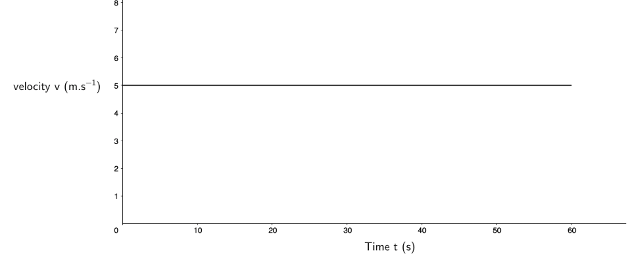
   The car is travelling at a constant positive velocity. Therefore, its acceleration is constant and zero and the increase in its displacement is a constant [latex]\scriptsize 5\ \text{m}[/latex] every second (the gradient of the displacement–time graph).
3. .
   1. .
      
   2. The velocity of the racing car after [latex]\scriptsize 30\ \text{s}[/latex] is [latex]\scriptsize 90\ \text{m}\text{.}{{\text{s}}^{{-1}}}[/latex].
   3. Area under the graph for the full [latex]\scriptsize 65\ \text{s}[/latex]:
      [latex]\scriptsize \left( {\displaystyle \frac{1}{2}\times 30\ \text{s}\times 90\ \text{m}\text{.}{{\text{s}}^{{\text{-1}}}}} \right)+\left( {20\ \text{s}\times 90\ \text{m}\text{.}{{\text{s}}^{{\text{-1}}}}} \right)+\left( {\displaystyle \frac{1}{2}\times 15\ \text{s}\times 90\ \text{m}\text{.}{{\text{s}}^{{\text{-1}}}}} \right)=3\ 825\ \text{m}[/latex]

Back to Unit 2: Assessment