Mechanics: State, explain and interpret principles of horizontal motion
Unit 3: More graphs of motion
Dylan Busa
Unit outcomes
By the end of this unit you will be able to:
- Analyse and interpret more complicated graphs of motion including:
- displacement–time graphs
- velocity–time graphs
- acceleration–time graphs.
What you should know
Before you start this unit, make sure you can:
- Draw simple graphs of motion including displacement–time graphs, velocity–time graphs and acceleration–time graphs. Refer to unit 2 if you need help with this.
- Interpret simple graphs of motion including displacement–time graphs, velocity–time graphs and acceleration–time graphs. Refer to unit 2 if you need help with this.
Introduction
In this unit you will learn how to draw and interpret more complicated graphs of motion that include situations of decreasing velocity and acceleration as well as negative displacement, velocity and acceleration.
Interpreting more complicated graphs of motion
The best way to explore these ideas is by looking at some worked examples.
Example 3.1
A subway train accelerates uniformly from rest to [latex]\scriptsize 30.0\ \text{km/h}[/latex] in the first [latex]\scriptsize 20\ \text{s}[/latex] of its journey between stops.
- Draw an accurate velocity–time graph of this situation.
- Use the graph to determine the uniform rate of acceleration.
- Draw an accurate acceleration–time graph of this situation.
- Draw an approximate displacement–time graph of this situation.
Solutions
- The first thing we should do is convert the velocity into standard units.
[latex]\scriptsize 30.0\ \text{km/h}=8.33\ \text{m}\text{.}{{\text{s}}^{{\text{-1}}}}[/latex]
.
We are told that the train accelerates uniformly i.e. at the same rate throughout the period. Therefore, we know that the gradient of the velocity–time graph will be constant. In other words, it will be a straight line. The train also starts from rest and reaches a velocity of [latex]\scriptsize 8.33\ \text{m}\text{.}{{\text{s}}^{{\text{-1}}}}[/latex] after [latex]\scriptsize 20\ \text{s}[/latex]. Therefore, the velocity–time graph will look as follows:
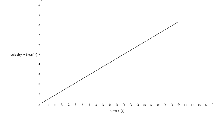
- To find the rate of acceleration, we have to measure the gradient of the velocity–time graph. Because the acceleration is uniform, we know the gradient of the line is the same for the whole line. Therefore, we can measure the gradient between any two convenient points, even the points at the start and end of the line.
.
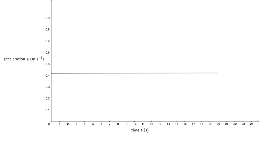
[latex]\scriptsize m=a=\displaystyle \frac{{{{v}_{f}}-{{v}_{i}}}}{{{{t}_{f}}-{{t}_{i}}}}=\displaystyle \frac{{8.33\ \text{m}\text{.}{{\text{s}}^{{\text{-1}}}}-0\ \text{m}\text{.}{{\text{s}}^{{\text{-1}}}}}}{{20\ \text{s}-0\ \text{s}}}=\displaystyle \frac{{8.33\ \text{m}\text{.}{{\text{s}}^{{\text{-1}}}}}}{{20\ \text{s}}}=0.427\ \text{m}\text{.}{{\text{s}}^{{\text{-2}}}}[/latex] - We know that the acceleration is a constant [latex]\scriptsize 0.43\ \text{m}\text{.}{{\text{s}}^{{\text{-2}}}}[/latex].
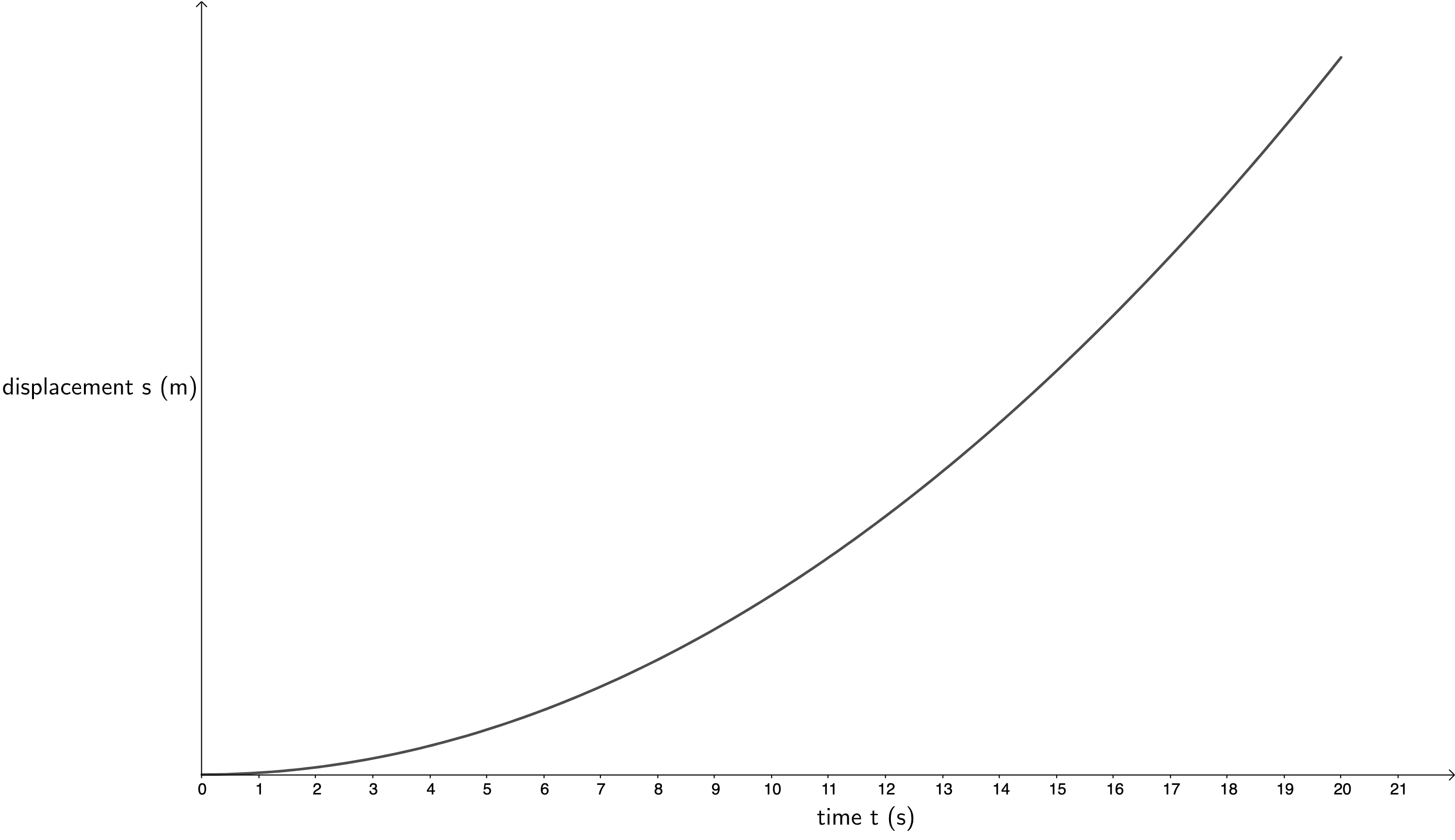
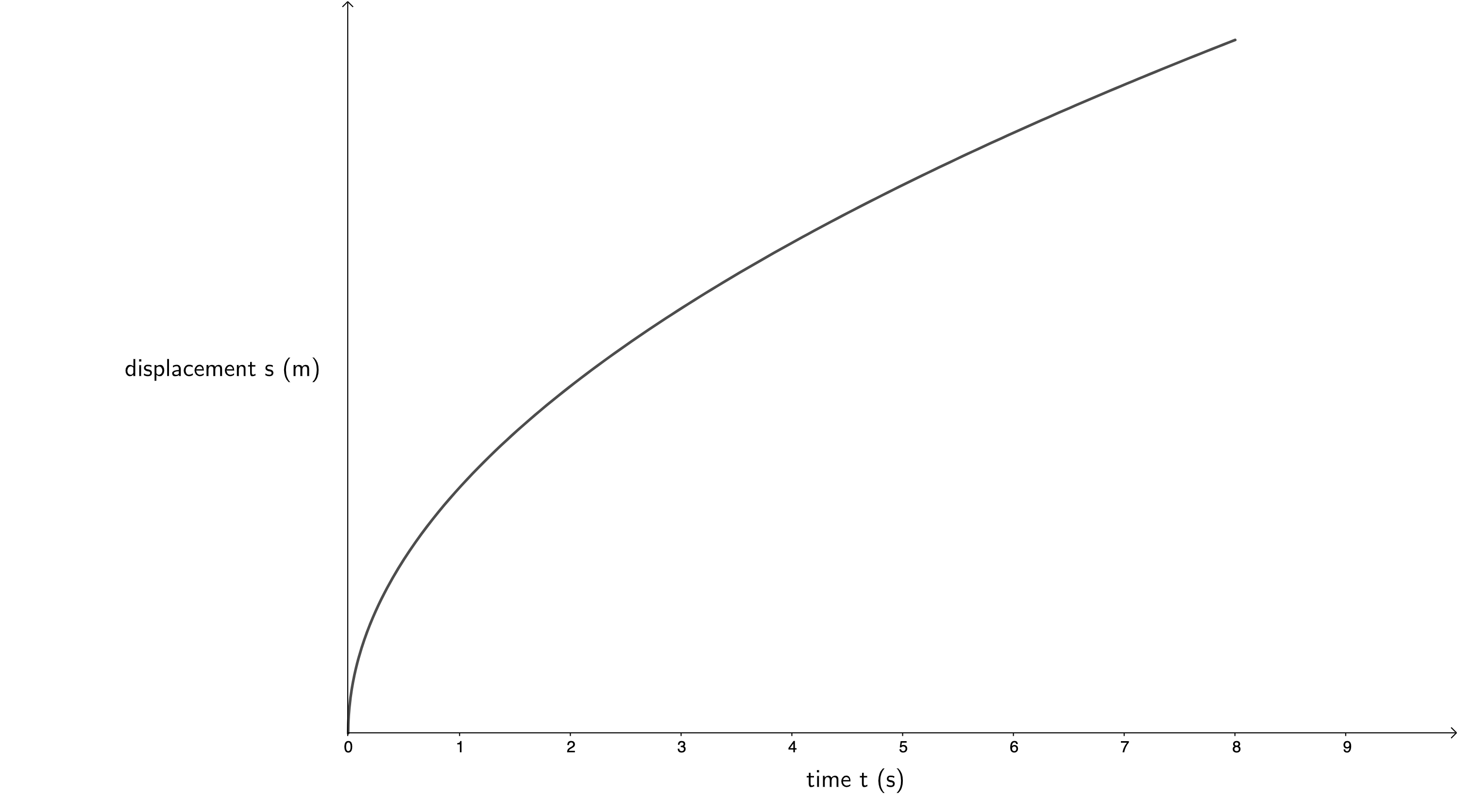
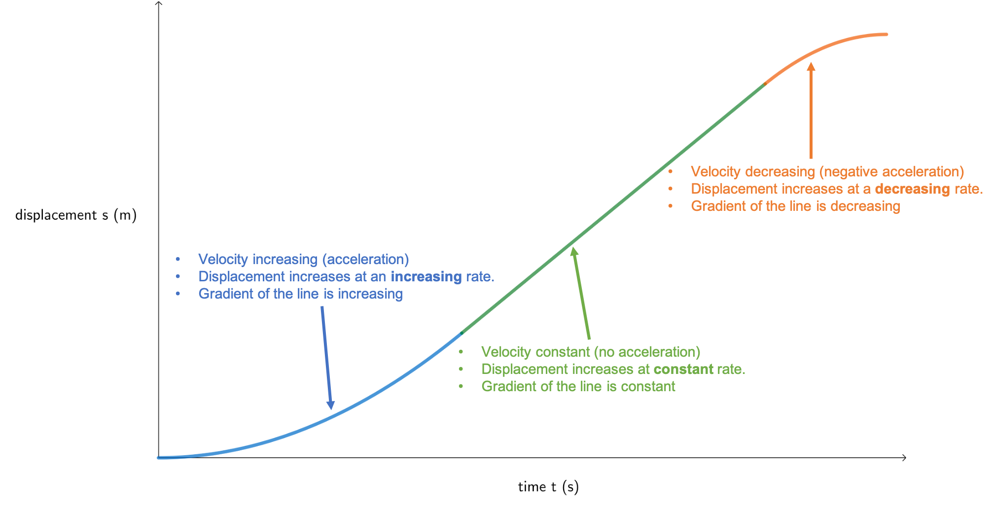
- For a body that is accelerating at a constant rate, its velocity is increasing as time passes and so its displacement is increasing at an increasing rate. In other words, the gradient of the displacement–time graph is not a straight line because a changing gradient reflects the changing velocity. As the velocity increases, the gradient of the displacement–time graph must also increase.
.
We have not added values to the y-axis because we do not know precisely what these are. We could use the equations of motion to calculate the maximum displacement of the train at [latex]\scriptsize 20\ \text{s}[/latex].
You should have found example 3.1 relatively simple as this is work we covered in unit 2. Work through example 3.2 now.
Example 3.2
Suppose the subway train from example 3.1 slows uniformly to a stop at the next station from a speed of [latex]\scriptsize 30.0\ \text{km/h}[/latex] in [latex]\scriptsize 8\ \text{s}[/latex].
- Draw an accurate velocity–time graph of this situation, taking the time when it starts to slow down as [latex]\scriptsize t=0\ \text{s}[/latex].
- Use the graph to determine the uniform rate of acceleration.
- Draw an accurate acceleration–time graph of this situation.
- Draw an approximate displacement–time graph of this situation.
- If between accelerating to [latex]\scriptsize 30.0\ \text{km/h}[/latex] and then decelerating to a stop again, the train travels at a constant velocity for [latex]\scriptsize 20\ \text{s}[/latex], draw velocity–time, acceleration–time and displacement–time graphs of the train’s entire journey from the first stop to the second.
Solutions
- In this case, the train’s velocity will decrease at a constant rate. Therefore, its gradient will be constant but negative. We know from example 3.1 that its initial velocity is [latex]\scriptsize 8.33\ \text{m}\text{.}{{\text{s}}^{{\text{-1}}}}[/latex].
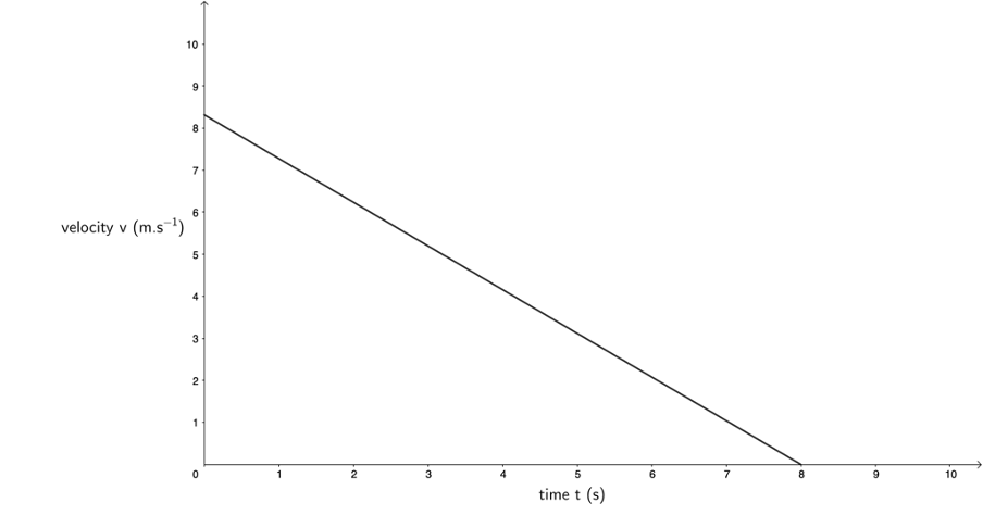
- To find the rate of acceleration, we have to measure the gradient of the velocity–time graph. Because the acceleration is uniform, we know the gradient of the line is the same for the whole line. Therefore, we can measure the gradient between any two convenient points, even the points at the start and end of the line. We can already see that, because the velocity–time graph gradient is negative, our acceleration will be negative (indicating deceleration).
.
[latex]\scriptsize m=a=\displaystyle \frac{{{{v}_{f}}-{{v}_{i}}}}{{{{t}_{f}}-{{t}_{i}}}}=\displaystyle \frac{{0\ \text{m}\text{.}{{\text{s}}^{{\text{-1}}}}-8.33\ \text{m}\text{.}{{\text{s}}^{{\text{-1}}}}}}{{8\ \text{s}-0\ \text{s}}}=\displaystyle \frac{{-8.33\ \text{m}\text{.}{{\text{s}}^{{\text{-1}}}}}}{{8\ \text{s}}}=-1.04\ \text{m}\text{.}{{\text{s}}^{{\text{-2}}}}[/latex] - We know that the acceleration is a constant [latex]\scriptsize -1.04\ \text{m}\text{.}{{\text{s}}^{{\text{-2}}}}[/latex].

- For a body that is decelerating at a constant rate, its velocity is decreasing as time passes and so its displacement is still increasing but at a decreasing rate. In other words, the gradient of the displacement–time graph is not a straight line because a changing gradient reflects the changing velocity. As the velocity decreases, the gradient of the displacement–time graph must also decrease.
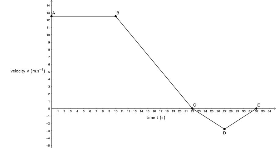
- Here is the velocity–time graph:
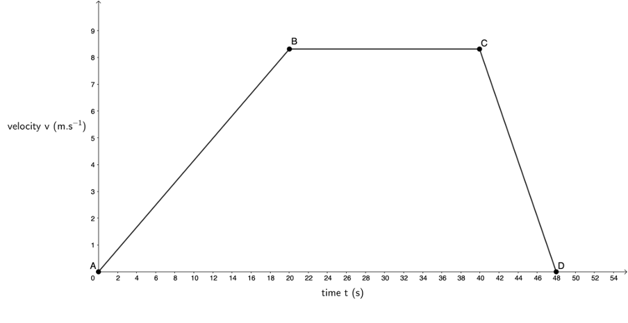
Between A and B, the train accelerated from [latex]\scriptsize 0\ \text{m}\text{.}{{\text{s}}^{{\text{-1}}}}[/latex] to [latex]\scriptsize 8.33\ \text{m}\text{.}{{\text{s}}^{{\text{-1}}}}[/latex]. Between B and C, the train travelled at a constant velocity of [latex]\scriptsize 8.33\ \text{m}\text{.}{{\text{s}}^{{\text{-1}}}}[/latex]. Between C and D, the train decelerated from [latex]\scriptsize 8.33\ \text{m}\text{.}{{\text{s}}^{{\text{-1}}}}[/latex] to [latex]\scriptsize 0\ \text{m}\text{.}{{\text{s}}^{{\text{-1}}}}[/latex].
.
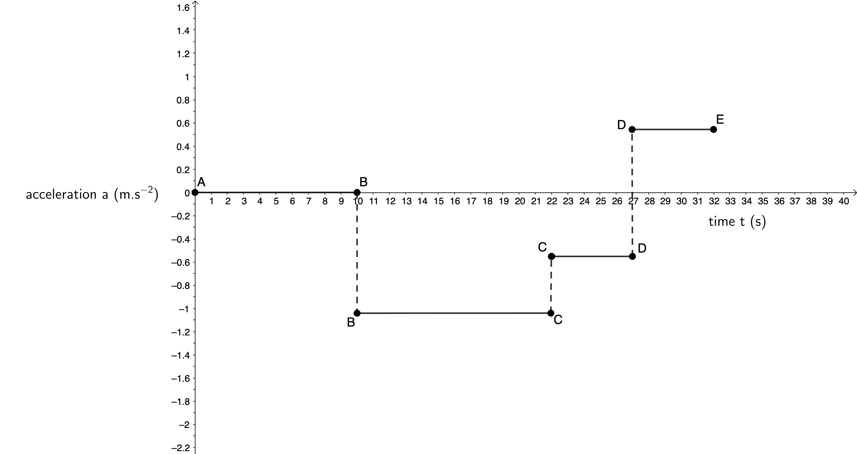
Here is the acceleration–time graph:
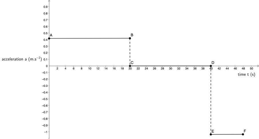
From A to B, the train accelerated at a constant rate of [latex]\scriptsize 0.43\ \text{m}\text{.}{{\text{s}}^{{\text{-2}}}}[/latex]. Between C and D, the train travelled at a constant velocity, hence its acceleration was [latex]\scriptsize 0\ \text{m}\text{.}{{\text{s}}^{{\text{-2}}}}[/latex]. Between E and F, the train accelerated at a constant rate of [latex]\scriptsize -1.04\ \text{m}\text{.}{{\text{s}}^{{\text{-2}}}}[/latex] (decelerated).
.
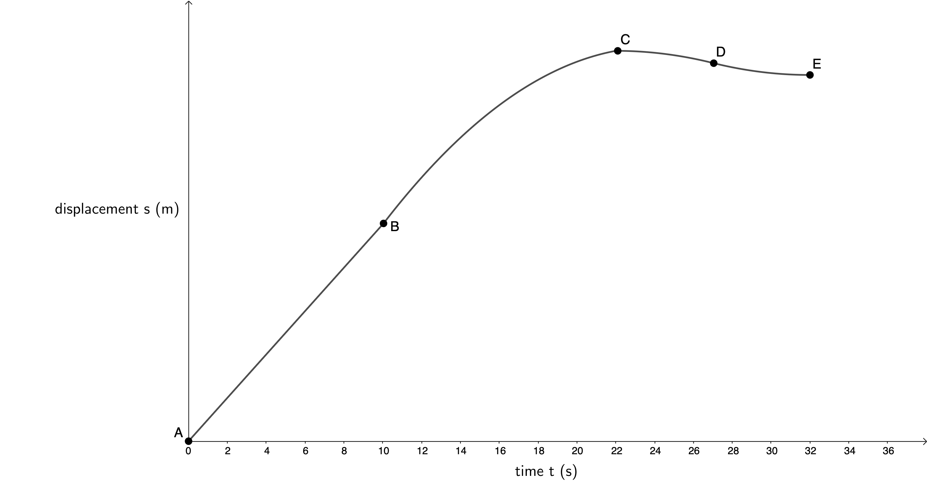
Here is the displacement–time graph:
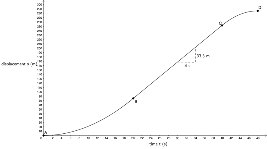
Between A and B, the train’s velocity was increasing. Therefore, the train’s displacement was increasing at an increasing rate. The total displacement after [latex]\scriptsize 20\ \text{s}[/latex] can be calculated as:
[latex]\scriptsize \begin{align*}s&=ut+\displaystyle \frac{1}{2}a{{t}^{2}}\\&=0\times 20\ \text{s}+\displaystyle \frac{1}{2}\times 0.43\ \text{m}\text{.}{{\text{s}}^{{-2}}}\times {{(20\ \text{s})}^{2}}\\&=86\ \text{m}\end{align*}[/latex]
.
Between B and C, the train travelled at a constant velocity of [latex]\scriptsize 8.33\ \text{m}\text{.}{{\text{s}}^{{\text{-1}}}}[/latex]. Therefore, the graph is a straight line with a positive gradient of [latex]\scriptsize 8.33\ \text{m}\text{.}{{\text{s}}^{{\text{-1}}}}[/latex]. The displacement after these [latex]\scriptsize 20\ \text{s}[/latex] can be calculated as:
[latex]\scriptsize \begin{align*}s&=ut+\displaystyle \frac{1}{2}a{{t}^{2}}\\&=8.33\ \text{m}\text{.}{{\text{s}}^{{-1}}}\times 20\ \text{s}+\displaystyle \frac{1}{2}\times 0\ \text{m}\text{.}{{\text{s}}^{{-2}}}\times {{(20\ \text{s})}^{2}}\\&=166.6\ \text{m}\end{align*}[/latex]
.
So, the train’s total displacement at this point is [latex]\scriptsize 86\ \text{m}+166.6\ \text{m}=252.6\ \text{m}[/latex].
.
Between C and D, the train’s velocity decreased and so its displacement increased but at a decreasing rate. The displacement during these [latex]\scriptsize 8\ \text{s}[/latex] can be calculated as:
[latex]\scriptsize \begin{align*}s&=ut+\displaystyle \frac{1}{2}a{{t}^{2}}\\&=8.33\ \text{m}\text{.}{{\text{s}}^{{-1}}}\times 8\ \text{s}+\displaystyle \frac{1}{2}\times \left( {-1.04\ \text{m}\text{.}{{\text{s}}^{{-2}}}} \right)\times {{(8\ \text{s})}^{2}}\\&=33.36\ \text{m}\end{align*}[/latex]
.
Therefore, the train’s total displacement at this point is:
[latex]\scriptsize 86\ \text{m}+166.6\ \text{m}+33.36\ \text{m}=285.96\ \text{m}[/latex]
.
Note: You will not be expected to draw an accurate displacement–time graph for this kind of situation. However, it is important that you understand why the graph is shaped like it is and to see the direct link between the graph and the equations of motion we covered in unit 1.
We can see from example 3.2 what the effects of negative acceleration are. At no point in the journey did the train travel ‘backwards’ towards the first station and so at no time is the velocity–time graph below the x-axis (negative velocity). However, as the acceleration during the final [latex]\scriptsize 8\ \text{s}[/latex] was negative, we represent this on the acceleration–time graph with a line below the x-axis.
It is also important to realise how the shape of the displacement–time graph changes from a situation with positive acceleration to one with negative acceleration. At no time does the train get closer to the first station (negative displacement). Its displacement from the first station is always increasing, however the rate of this increase increases during the first [latex]\scriptsize 20\ \text{s}[/latex], remains constant during the next [latex]\scriptsize 20\ \text{s}[/latex] and decreases during the last [latex]\scriptsize 8\ \text{s}[/latex] (see figure 1).
Example 3.3
A subway train approaches a station travelling at a constant velocity of [latex]\scriptsize 45\ \text{km/h}[/latex]. After [latex]\scriptsize 10\ \text{s}[/latex], it decelerates uniformly to rest in [latex]\scriptsize 12\ \text{s}[/latex]. Unfortunately, it overshoots the station and has to reverse, which it does so immediately, accelerating uniformly to [latex]\scriptsize 10\ \text{km/h}[/latex] in [latex]\scriptsize 5\ \text{s}[/latex] and then immediately decelerating to rest at the station in [latex]\scriptsize 5\ \text{s}[/latex].
- Draw an accurate velocity–time graph of this situation.
- Draw an accurate acceleration–time graph of this situation.
- Draw an approximate displacement–time graph of this situation.
- Use one of your graphs to determine the distance the train had to reverse back to the station.
Solutions
Before we begin answering any of the questions, we need to define the positive direction for all our vectors. We will assign the initial direction the train travelled to the station as the positive direction and the direction it travelled while reversing back to the station as the negative direction.
- [latex]\scriptsize 45\ \text{km/h}=12.5\ \text{m}\text{.}{{\text{s}}^{{\text{-1}}}}[/latex]
[latex]\scriptsize 10\ \text{km/h}=2.78\ \text{m}\text{.}{{\text{s}}^{{\text{-1}}}}[/latex]
The velocity–time graph is as follows:
Between A and B, the train is travelling at a constant speed of [latex]\scriptsize 12.5\ \text{m}\text{.}{{\text{s}}^{{\text{-1}}}}[/latex] for [latex]\scriptsize 10\ \text{s}[/latex]. Between B and C, the train is decelerating uniformly to rest (hence the gradient of the line is constant but negative). From C to D, the train is accelerating to [latex]\scriptsize 2.78\ \text{m}\text{.}{{\text{s}}^{{\text{-1}}}}[/latex]. However, this is in the negative direction. So, the actual velocity reached after [latex]\scriptsize 5\ \text{s}[/latex] of uniform acceleration is [latex]\scriptsize -2.78\ \text{m}\text{.}{{\text{s}}^{{\text{-1}}}}[/latex] and the graph is below the x-axis. From D to E the train is decelerating uniformly to rest in [latex]\scriptsize 5\ \text{s}[/latex]. During this period, the train is still travelling in the negative direction and so the graph is below the x-axis. - The acceleration–time graph is as follows:
Between A and B, the train is travelling at a constant velocity. Therefore, the acceleration is zero. The gradient of the velocity–time graph during this period is zero. Between B and C, the train is decelerating to rest at [latex]\scriptsize -1.04\ \text{m}\text{.}{{\text{s}}^{{\text{-2}}}}[/latex]. The acceleration for this period is negative and so is drawn below the x-axis. We can see that the gradient of the velocity–time graph is constant and negative during this period. Between C and D the train is accelerating from rest to [latex]\scriptsize 2.78\ \text{m}\text{.}{{\text{s}}^{{\text{-1}}}}[/latex]. It may seem strange, however, that this part of the graph is also negative. If you look at the velocity-time graph for this period (C to D), you will see that its gradient is a constant but negative [latex]\scriptsize 0.56\ \text{m}\text{.}{{\text{s}}^{{\text{-2}}}}[/latex]. Even though the train is accelerating (which we normally take to be positive acceleration), it is accelerating in the negative direction. Therefore, this acceleration is [latex]\scriptsize -0.56\ \text{m}\text{.}{{\text{s}}^{{\text{-2}}}}[/latex].
.
Between D and E, the train is decelerating to rest. This is in the negative direction so we can think of this deceleration as [latex]\scriptsize -\left( {-0.56\ \text{m}\text{.}{{\text{s}}^{{\text{-2}}}}} \right)=0.56\ \text{m}\text{.}{{\text{s}}^{{\text{-2}}}}[/latex] i.e. a positive acceleration. We can also see that during this period, the gradient of the velocity–time graph is constant and positive. Therefore, this part of the acceleration–time graph is above the x-axis. - The displacement–time graph has the following shape:
Between A and B, the train is travelling at a constant velocity of [latex]\scriptsize 12.5\ \text{m}\text{.}{{\text{s}}^{{\text{-1}}}}[/latex]. Therefore, the displacement–time graph has a constant positive gradient of [latex]\scriptsize 12.5\ \text{m}\text{.}{{\text{s}}^{{\text{-1}}}}[/latex]. Between B and C, the train is decelerating but still travelling in the positive direction. Therefore, its displacement is still increasing but at a decreasing rate as the velocity decreases. Therefore, the displacement–time graph gradient is decreasing. Between C and D, the train starts reversing. Therefore, its displacement is decreasing. Its velocity is negative and increasing and so the gradient of the displacement–time graph is negative and getting more negative. From D to E, the train slows down but is still travelling in the negative direction. Therefore, displacement is still decreasing but at a slower rate as the negative velocity is decreasing and so the gradient of the displacement–time graph is negative but getting less negative. - The best graph to use is the velocity–time graph. We need to calculate the area under the graph between points C and E to determine how far the train needed to travel in reverse to get back to the station.
.
We need to split this area into two triangles. Both will have a base of [latex]\scriptsize 5\ \text{s}[/latex] and a vertical height of [latex]\scriptsize 2.78\ \text{m}\text{.}{{\text{s}}^{{\text{-1}}}}[/latex]. Because we are calculating area, we do not need to take the negative nature of the velocity into account.
.
[latex]\scriptsize \displaystyle \text{Area}=2\times \displaystyle \frac{1}{2}\times 5\ \text{s}\times 2.78\ \text{m}\text{.}{{\text{s}}^{{\text{-1}}}}=13.9\ \text{m}[/latex]
Therefore, the train missed the station by [latex]\scriptsize \displaystyle 13.9\ \text{m}[/latex].
The most important thing to note about these examples is the signs of the vectors as reflected by the gradients of the graphs, and whether the graphs are above (positive) or below (negative) the x-axis.
In example 3.3 our chosen positive direction was initially towards the station. Therefore, the initial velocities were positive and the fact that the initial acceleration was negative made sense. Most people interpret negative acceleration as the slowing of an object (deceleration).
However, this was not always the case in example 3.3. A negative acceleration increased a negative velocity, and a positive acceleration decreased a negative velocity. The crucial point is that the acceleration was in the opposite direction from the velocity. A negative acceleration increases a negative velocity.
A good general rule is this:
If acceleration has the same sign as the velocity, the object is speeding up. If acceleration has the opposite sign to the velocity, the object is slowing down.
Exercise 3.1
Question 1 adapted from NC(V) Physical Science Level 3 Paper 1 February 2019 question 4.3
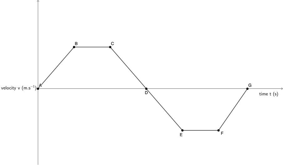
- Consider the following displacement–time graph given below for the motion of a bus:

- Which statement is true?
Between D and E:- The bus is accelerating in the forward direction.
- The bus is accelerating in the reverse direction.
- The bus is decelerating in the forward direction.
- The bus is decelerating in the reverse direction.
- Describe the acceleration of the bus between B and C.
- Describe the motion of the bus between E and G.
- Draw a velocity–time graph for this situation labelling the different portions A to G to correspond with the displacement–time graph.
- Draw an acceleration–time graph for this situation labelling the different portions A to G to correspond with the displacement–time graph.
- Which statement is true?
- The acceleration–time graph for an electric vehicle starting from rest, is given below:
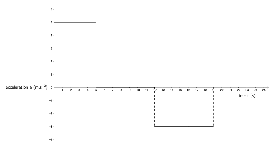
- Calculate the velocity of the car and hence draw the velocity–time graph.
- Use a graph to determine the total displacement of the vehicle.
The full solutions can be found at the end of the unit.
Summary
In this unit you have learnt the following:
- Objects with a constant positive acceleration have a displacement–time graph with an increasing gradient. If the velocity is positive, the displacement increases over time.
- Objects with a constant negative acceleration have a displacement–time graph with a decreasing gradient. If the velocity is negative, the displacement decreases over time.
- If acceleration has the same sign as the velocity, the object is speeding up.
- If acceleration has the opposite sign as the velocity, the object is slowing down.
Unit 3: Assessment
Suggested time to complete: 30 minutes
Question 1 adapted from NC(V) Physical Science Level 3 Paper 1 November 2019 question 6
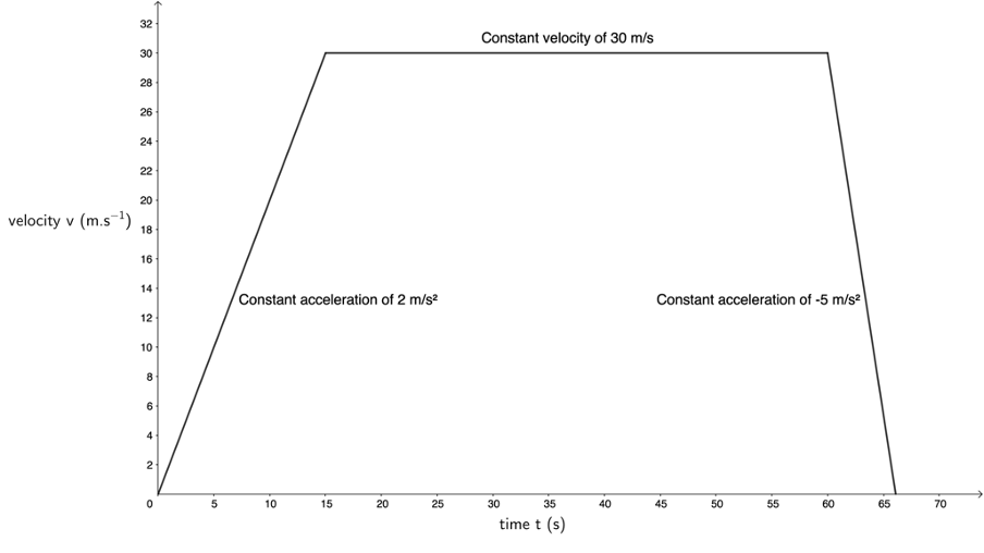
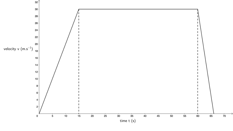
- A bus starts from rest at a station and accelerates at a rate of [latex]\scriptsize \displaystyle 2\ \text{m}\text{.}{{\text{s}}^{{-2}}}[/latex] for [latex]\scriptsize \displaystyle 15\ \text{s}[/latex]. It then travels at a constant speed for [latex]\scriptsize \displaystyle 45\ \text{s}[/latex] and slows down at a rate of [latex]\scriptsize \displaystyle 5\ \text{m}\text{.}{{\text{s}}^{{-2}}}[/latex] until it comes to a stop.
- Determine the velocity of the bus after [latex]\scriptsize \displaystyle 15\ \text{s}[/latex]?
- [latex]\scriptsize 60~\text{s}[/latex] after leaving the station, the bus starts to slow down. How much time does the bus take to slow down and come to a stop?
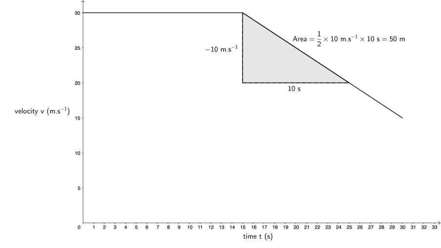
- Draw a velocity–time graph for the motion of the bus. Indicate ALL details on the graph.
- From the graph, determine the distance covered by the bus (i.e. do not use equations of motion).
Question 2 adapted from NC(V) Physical Science Level 3 Paper 1 February 2019 question 6.2
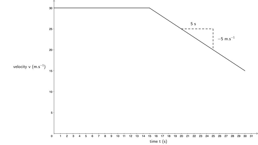
- After travelling at [latex]\scriptsize \displaystyle 30\ \text{m}\text{.}{{\text{s}}^{{-1}}}[/latex] for [latex]\scriptsize \displaystyle 15\ \text{s}[/latex], the driver of a car sees a traffic camera [latex]\scriptsize \displaystyle 50\ \text{m}[/latex] away. The driver knows the speed limit is [latex]\scriptsize \displaystyle 60\ \text{km/h}[/latex], so she accelerates at [latex]\scriptsize \displaystyle -1\ \text{m}\text{.}{{\text{s}}^{{-2}}}[/latex] until her velocity is [latex]\scriptsize \displaystyle 54\ \text{km/h}[/latex].
- Draw a velocity–time graph depicting her motion to the point she passes the camera.
- Use your graph to determine her velocity when she passes the camera.
- Is the driver travelling above or below the speed limit when she passes the camera?
The full solutions can be found at the end of the unit.
Unit 3: Solutions
Exercise 3.1
- .
- ii. (Between D and E the bus is accelerating in the reverse direction).
- Between B and C, the bus is travelling with constant positive velocity. Therefore, its acceleration is zero.
- Between E and F, the bus is travelling with constant negative velocity. Therefore, its acceleration is zero. However, between F and G, its negative velocity is decreasing to zero. Therefore, the bus is accelerating with positive acceleration.
- .
- .
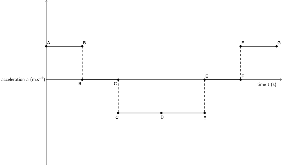
- .
- The area under an acceleration–time graph gives the velocity.
[latex]\scriptsize \displaystyle t=0\ \text{s}[/latex] to [latex]\scriptsize \displaystyle t=5\ \text{s}[/latex]: [latex]\scriptsize \text{Area}=5\ \text{m}\text{.}{{\text{s}}^{{\text{-2}}}}\times 5\ \text{s}=25\ \text{m}\text{.}{{\text{s}}^{{\text{-1}}}}[/latex] Therefore, the vehicle’s velocity after [latex]\scriptsize \displaystyle 5\ \text{s}[/latex] is [latex]\scriptsize 25\ \text{m}\text{.}{{\text{s}}^{{\text{-1}}}}[/latex].
.
[latex]\scriptsize \displaystyle t=5\ \text{s}[/latex] to [latex]\scriptsize \displaystyle t=12\ \text{s}[/latex]: acceleration is zero. Therefore, the vehicle’s velocity is constant i.e. [latex]\scriptsize {{v}_{f}}={{v}_{i}}[/latex] and its velocity after [latex]\scriptsize \displaystyle 12\ \text{s}[/latex] is still [latex]\scriptsize 25\ \text{m}\text{.}{{\text{s}}^{{\text{-1}}}}[/latex].
.
[latex]\scriptsize \displaystyle t=12\ \text{s}[/latex] to [latex]\scriptsize \displaystyle t=19\ \text{s}[/latex]: [latex]\scriptsize \text{Area}=-3\ \text{m}\text{.}{{\text{s}}^{{\text{-2}}}}\times 7\ \text{s}=-21\ \text{m}\text{.}{{\text{s}}^{{\text{-1}}}}[/latex] Therefore, if the vehicle’s initial velocity is [latex]\scriptsize 25\ \text{m}\text{.}{{\text{s}}^{{\text{-1}}}}[/latex] at [latex]\scriptsize \displaystyle t=12\ \text{s}[/latex], its final velocity will be [latex]\scriptsize 4\ \text{m}\text{.}{{\text{s}}^{{\text{-1}}}}[/latex] at [latex]\scriptsize \displaystyle t=19\ \text{s}[/latex].
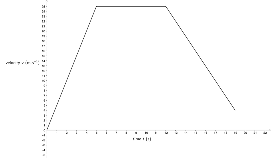
- The area under the velocity–time graph gives total displacement. The image below shows one way of dividing up the area under the velocity–time graph.
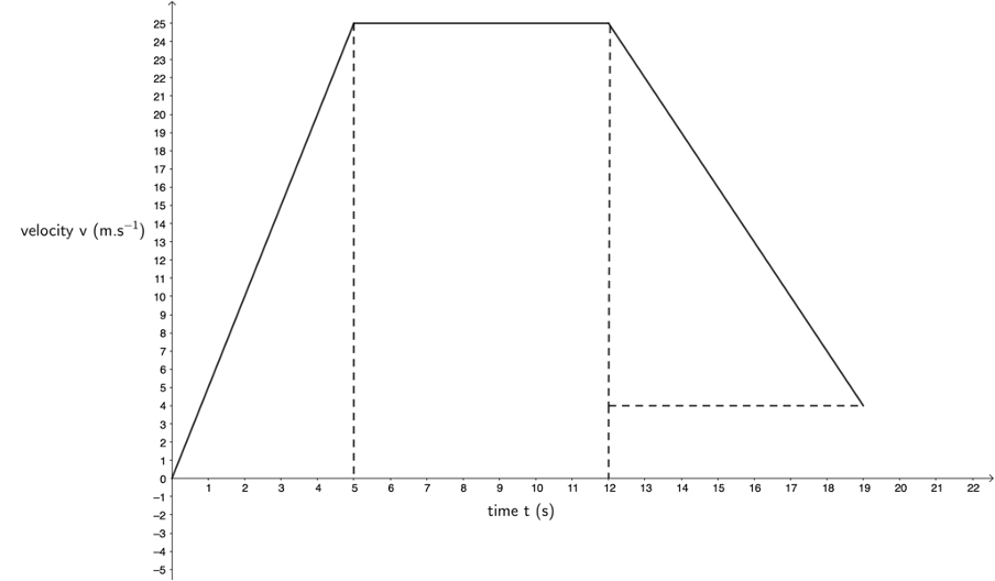
[latex]\scriptsize \text{Total displacement}=\left( {\displaystyle \frac{1}{2}\times 25\ \text{m}\text{.}{{\text{s}}^{{\text{-1}}}}\times 5\ \text{s}} \right)+\left( {25\ \text{m}\text{.}{{\text{s}}^{{\text{-1}}}}\times 7\ \text{s}} \right)+\left( {\displaystyle \frac{1}{2}\times 21\ \text{m}\text{.}{{\text{s}}^{{\text{-1}}}}\times 7\ \text{s}} \right)=311\ \text{m}[/latex]
- The area under an acceleration–time graph gives the velocity.
Unit 3: Assessment
- .
- .
[latex]\scriptsize \begin {align*} v&=u+at\\ \therefore v&=0~\text{m.s}^{-1}+2~\text{m.s}^{-2} \times 15~\text{s}=30~\text{m.s}^{-1} \end {align*}[/latex] - .
[latex]\scriptsize \begin {align*} v&=0~\text{m.s}^{-1}\\ u&=30~\text{m.s}^{-1}\\ a&=-5~\text{m.s}^{-2}\\ t&=?\\ v&=u+at\\ \therefore t&=\displaystyle \frac{v-u}{a}\\ &=\displaystyle \frac{0~\text{m.s}^{-1}-30~\text{m.s}^{-1}}{-5~\text{m.s}^{-2}}\\ &=6~\text{s} \end {align*}[/latex] - .
- .
[latex]\scriptsize \begin {align*} \text{Total displacement}&=\displaystyle \frac{1}{2}\times 30~\text{m.s}^{-1}\times 15~\text{s}+30~\text{m.s}^{-1}\times 45~\text{s}+\displaystyle \frac{1}{2}\times 30~\text{m.s}^{-1}\times 6~\text{s}\\ &=1~665~\text{m} \end {align*}[/latex]
- .
- .
- Initial velocity is [latex]\scriptsize 30~\text{m.s}^{-1}[/latex]. Final velocity is [latex]\scriptsize 54~\text{km/h}=15~\text{m.s}^{-1}[/latex].
- The driver travels [latex]\scriptsize 50~\text{m}[/latex] before passing the camera. Therefore, we need to find the section with an area of [latex]\scriptsize 50~\text{m}[/latex] under the part of the velocity–time graph indicating deceleration.
[latex]\scriptsize \begin {align*} \text{Area}&=\displaystyle \frac{1}{2}\times \text{base}\times\text{height}\\ \therefore \text{base}\times\text{height}&=100 \end {align*}[/latex]
.
But the gradient of the line is [latex]\scriptsize -1~\text{m.s}^{-2}[/latex]. Therefore, the change in [latex]\scriptsize x[/latex] will be the same as the change in [latex]\scriptsize y[/latex].
.
Therefore [latex]\scriptsize \text{base}=\text{height}=\sqrt{100}=10[/latex].
.
This means that the driver will travel for [latex]\scriptsize 10~\text{s}[/latex] while accelerating at [latex]\scriptsize -1~\text{m.s}^{-2}[/latex].
The driver’s velocity after [latex]\scriptsize 10~\text{s}[/latex] will be [latex]\scriptsize 20~\text{m.s}^{-1}[/latex] when the car passes the camera. - [latex]\scriptsize 20~\text{m.s}^{-1}=72~\text{km/h}[/latex]. She will still be over the speed limit when she passes the camera.
- Initial velocity is [latex]\scriptsize 30~\text{m.s}^{-1}[/latex]. Final velocity is [latex]\scriptsize 54~\text{km/h}=15~\text{m.s}^{-1}[/latex].
Media Attributions
- example3.1A1 © Geogebra is licensed under a CC BY-SA (Attribution ShareAlike) license
- example3.1A3 © Geogebra is licensed under a CC BY-SA (Attribution ShareAlike) license
- example3.1A4 © Geogebra is licensed under a CC BY-SA (Attribution ShareAlike) license
- example3.2A1 © Geogebra is licensed under a CC BY-SA (Attribution ShareAlike) license
- example3.2A3 © Geogebra is licensed under a CC BY-SA (Attribution ShareAlike) license
- example3.2A4 © Geogebra is licensed under a CC BY-SA (Attribution ShareAlike) license
- example3.2A5.1 © Geogebra is licensed under a CC BY-SA (Attribution ShareAlike) license
- example3.2A5.2 © Geogebra is licensed under a CC BY-SA (Attribution ShareAlike) license
- example3.2A5.3 © Geogebra is licensed under a CC BY-SA (Attribution ShareAlike) license
- figure1 © DHET is licensed under a CC BY (Attribution) license
- example3.3A1 © Geogebra is licensed under a CC BY-SA (Attribution ShareAlike) license
- example3.3A2 © Geogebra is licensed under a CC BY-SA (Attribution ShareAlike) license
- example3.3A3 © Geogebra is licensed under a CC BY-SA (Attribution ShareAlike) license
- exercise3.1Q1 © DHET is licensed under a CC BY (Attribution) license
- exercise3.1Q2 © Geogebra is licensed under a CC BY-SA (Attribution ShareAlike) license
- exercise3.1A1d © Geogebra is licensed under a CC BY-SA (Attribution ShareAlike) license
- exercise3.1A1e © Geogebra is licensed under a CC BY-SA (Attribution ShareAlike) license
- exercise3.1A2a © Geogebra is licensed under a CC BY-SA (Attribution ShareAlike) license
- exercise3.1A2b © Geogebra is licensed under a CC BY-SA (Attribution ShareAlike) license
- assessmentA1c © Geogebra is licensed under a CC BY-SA (Attribution ShareAlike) license
- assessmentA1d © Geogebra is licensed under a CC BY-SA (Attribution ShareAlike) license
- assessmentA2a © Geogebra is licensed under a CC BY-SA (Attribution ShareAlike) license
- assessmentA2b © Geogebra is licensed under a CC BY-SA (Attribution ShareAlike) license
